2D Boundary Conditions Editor

Configure boundary conditions in the 2D Boundary Conditions editor (Boundary Conditions|2D Boundary Conditions).

If the 2D domain source is 'Domain file created from MIKE+ definition', the user must pre-define open 2D boundaries in the computation grid/mesh on the Map before configuring in the 2D Boundary Conditions editor. If the 2D domain source is 'Existing domain file', then the open 2D boundaries are identified from the selected flexible mesh file, and their locations cannot be modified in MIKE+.

By default, the 2D model is initially assigned a closed boundary, wherein water will not enter or leave the domain across its perimeter. However, it is possible to locally define other types of 2D hydrodynamic boundaries:

• Discharge: To define known discharge (constant or time varying) conditions along the boundary, such as where the 2D model perimeter crosses a river or similar.
• Water Level: Typically applied where the 2D model perimeter crosses a larger water body, such as a lake or the sea, where the water level is known (constant or time varying).
• Q/h Relation: A rating curve may be used to describe varying water level at the boundary as a function of the incoming discharge. May be used when the relationship between the discharge and the water level is known for the model.
• Free Outflow: Boundary condition type where water can freely leave the 2D domain across its perimeter.
• Source: To define local sources (or sinks) within the 2D domain.
• Closed: Boundary condition type where water will not enter or leave the 2D domain across its perimeter.

Closed boundary conditions are maintained along domain perimeter sections where no other boundary condition types are specified.

Each boundary section must span at least 2 grid/mesh nodes, and open boundary conditions require wet boundary sections.

The available options and tabs in the 2D Boundary Conditions editor vary depending on the type of boundary condition being set-up.

 

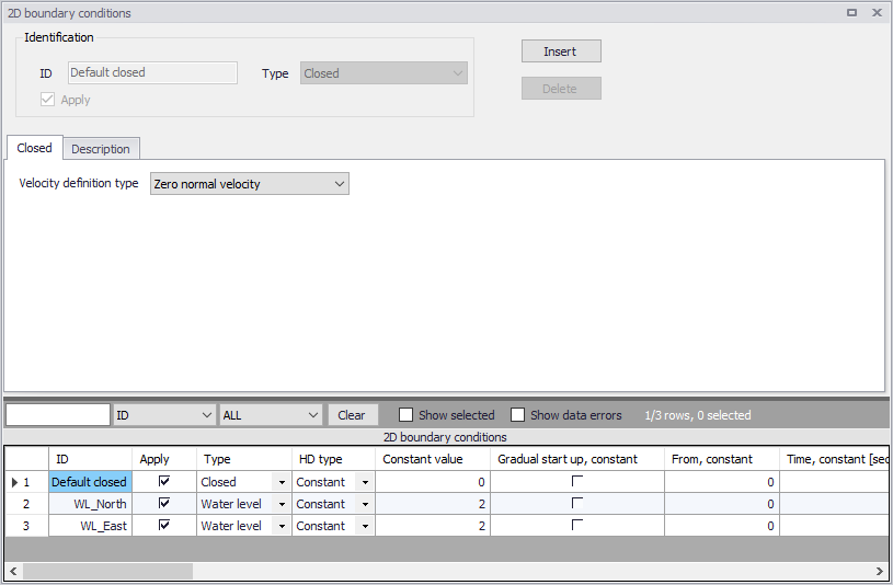
Figure: The 2D Boundary Conditions editor

Note

The location of source boundary conditions is defined or edited using the coordinates defined in the '2D boundary conditions' editor. It is different for the other types of boundary conditions which must always be drawn or edited on the map. Therefore, it is not possible to change a source boundary to another type of boundary condition, from the 'Type' list.

Defining 2D Boundary Conditions

Example workflows for setting up 2D boundary conditions in MIKE+ are described in the following sections.

For Newly-created Domain Grids/Meshes

This workflow is relevant for when new domain grids/meshes are being created in MIKE+ (i.e. Source = Domain file from MIKE+ definition).

Ensure the new domain grid/mesh has been generated e.g. following instructions in chapter 2D Domain.

Define 2D model boundary sections on the Map via the Edit Features toolbox on the 2D Overland menu ribbon (figure below) or the Flooding layer editing tools toolbar on the Map. Use the ‘Create’ tool to draw features on the Map. Click on mesh/grid nodes to locate the boundary condition. Right-click to remove the last vertex added, and double-click to finish drawing.

 

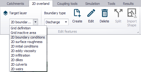
Figure: The Edit features toolbox on the 2D Overland menu ribbon

 

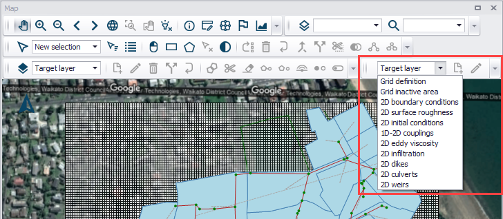
Figure: The Flooding Layer Editing Tools toolbar on the Map

1. Configure boundary conditions in the 2D Boundary Conditions Editor (Boundary Conditions|2D Boundary Conditions). Details on the various configuration parameters for each type of boundary condition are described in succeeding sections.

For Loaded Existing Domain Grids/Meshes

Specify the existing domain file for the 2D model in the 2D Overland editor.

When existing domain grids/meshes are loaded into MIKE+ (i.e. Source = Existing domain file), the program automatically detects any existing boundary definitions in the grid or mesh, and adds corresponding records to the 2D Boundary Conditions table.

Grid files have intrinsic information on boundary sections, wherein grid perimeter cells with (Bathymetry) values less than the ‘Land value’ are considered open boundaries (see figure below). These information may be checked by viewing the *.DFS2 grid file in the Grid Editor.

Viewing rectangular grids in the Grid Editor from MIKE+ is offered via the ellipsis button beside the ‘File path’ parameter in the 2D Domain editor, or using the ‘Grid editor’ tool in the ‘2D Domain Editors’ toolbox on the ‘2D Overland’ menu ribbon.

 

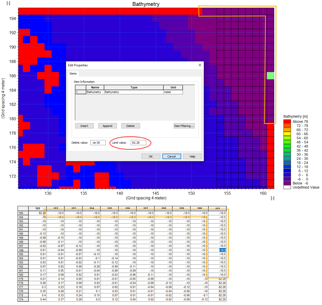
Figure: Rectangular grid file viewed in the Grid Editor showing the ‘Land value’ property (encircled in red) in the Edit Properties dialog (Edit|Items). Grid values are shown on the map as well as on the overview table, and the open boundary sections are outlined in yellow.

Mesh files also have built-in information about boundary sections; in this case via ‘Code value’ properties at element nodes (see figure below). These information may be checked by viewing the *.MESH file in the Data Viewer.

The ‘Code value’ is used to distinguish between the different boundary sections in the mesh. A value of ‘1’ is used for all closed boundaries, whereas all other open boundaries must be defined with a number >1.

Viewing meshes in the Data Viewer from MIKE+ is offered via the ellipsis button beside the ‘File path’ parameter in the 2D Domain editor, or using the ‘Data Viewer’ tool in the ‘2D Domain Editors’ toolbox on the ‘2D Overland’ menu ribbon.

 

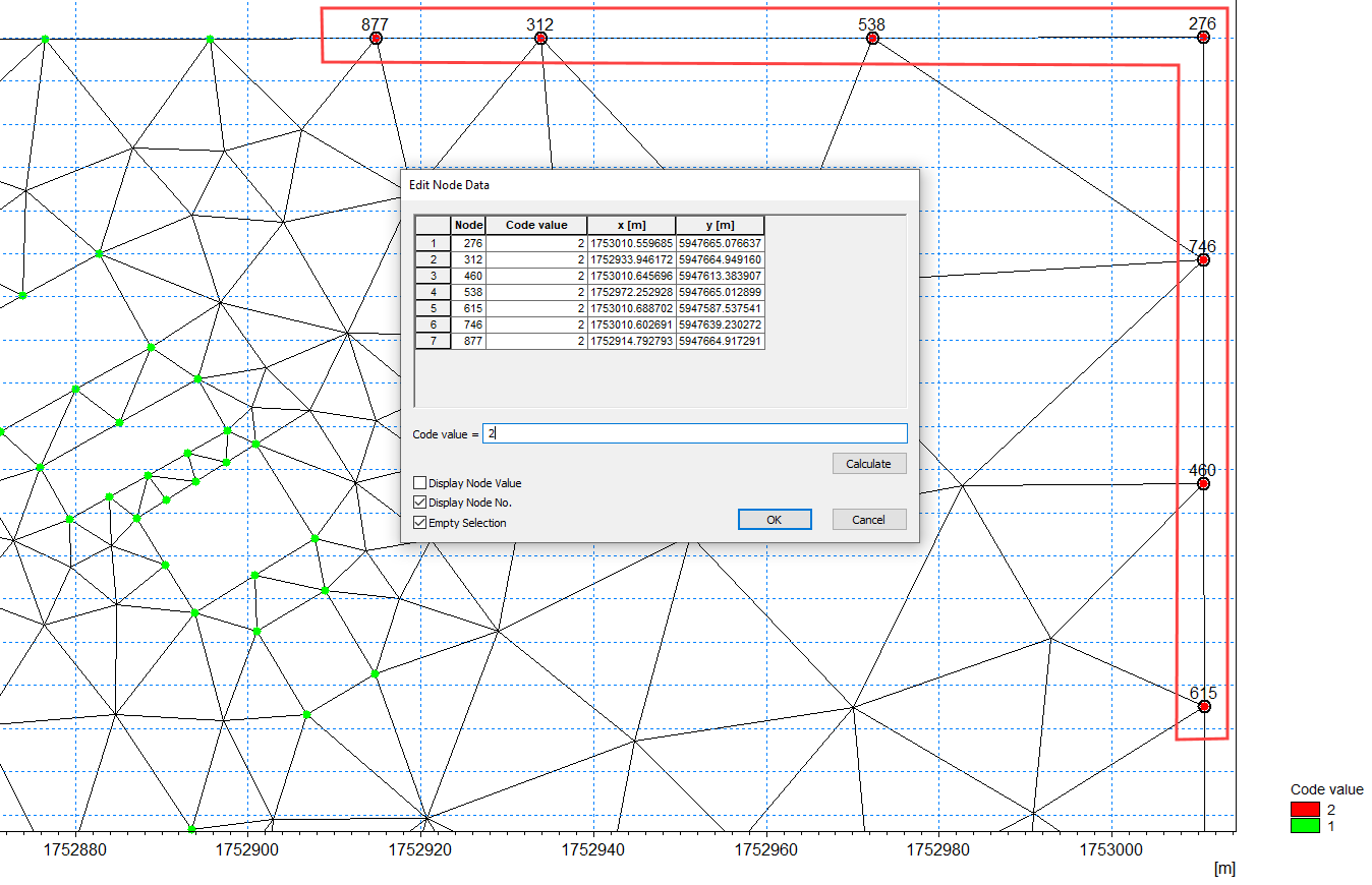
Figure: Mesh file viewed in the Data Viewer showing the ‘Code value’ properties for mesh perimeter nodes (outlined in red). Code values may be shown on the map by activating the corresponding data layer from the toolbar, or by selecting node points from the map.

Configure all the defined boundary conditions in the 2D Boundary Conditions Editor (Boundary Conditions|2D Boundary Conditions) (Figure 4.1). Details on the various configuration parameters for each type of boundary condition are described in succeeding sections.

Closed Boundaries

A closed boundary is first assigned the 2D domain perimeter by default. A closed boundary indicates water will not enter or leave the model domain across its perimeter. Closed boundaries can be of two types:

• Zero normal velocity: The default closed boundary type for 2D models in MIKE+. For this type, the free-slip boundary condition is assumed, wherein the normal velocity component is zero.
• Zero velocity: For this type, the no-slip boundary condition is assumed where both the normal and tangential velocity components are zero.

User-defined and local boundary conditions can also be set to be closed, for example to temporarily deactivate the boundary condition.

Discharge Boundaries

Temporal variation

Discharge boundary conditions can be constant in time, or vary as specified in a *.dfs0 timeseries file:

• Constant
• Varying in time: Requires a .dfs0 timeseries file of discharge that covers the entire simulation period. The time step of the input data file does not have to be the same as the time step of the hydrodynamic simulation.

An option for controlling the application of the boundary condition at the start of the simulation is offered via the ‘Gradual start up’ option. One may specify a soft start interval during which boundary values are increased from a specified reference value to the specified boundary value in order to avoid shock waves being generated in the model.

Discharge values shall either be positive or negative depending on the desired direction of the boundary (i.e. inflow or outflow).

Interpolation

For time-varying discharge boundaries, the interpolation method for determining values between available time step values in the specified file may be specified as Linear or Piecewise cubic in the ‘Interpolation’ tab. Also see section Interpolation types for more details.

The distribution of the total flow in the individual grid points along the boundary is calculated relative to the depth. The discharge is distributed as in a uniform flow field with the Manning resistance law applied, i.e. is relative to \(h^{5/3}\), where \(h\) is the depth.

 

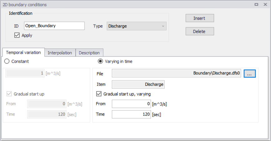
Figure: Set-up parameters for Discharge 2D Boundary Conditions

Water Level Boundaries

Temporal variation

Water level boundaries may be constant, time-varying, or temporally- and spatially-varying along the boundary line:

• Constant
• Varying in time: Requires a *.DFS0 timeseries file of water level that covers the entire simulation period. The time step of the input data file does not have to be the same as the time step of the hydrodynamic simulation.
• Varying in domain and time: Requires a *.DFS1 profile timeseries file.

Interpolation

For time-varying and space-varying water level boundaries, the interpolation method for determining values between available time step values in the specified file may be specified as Linear or Piecewise cubic in the ‘Interpolation’ tab.

For space-varying water level boundaries, mapping input data to the boundary section may also be specified as Clockwise or Counter-clockwise in the ‘Interpolation’ tab.

More details on options for interpolating and mapping the input data file to the boundary section are found under section Interpolation types.

 

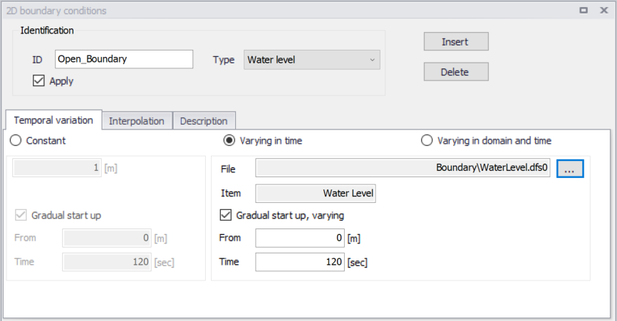
Figure: Parameters for Water Level 2D Boundary Conditions

Q/h Relation

This type of boundary is only recommended for downstream boundaries where water flows out of the 2D model.

The rating curve comprises of water level and discharge value pairs. The water level value is determined from the rating curve table using the appropriate discharge in the adjacent cells.

Define a table containing the relation between discharge and water level in the secondary table on the Q/h Relation tab page on the editor.

 

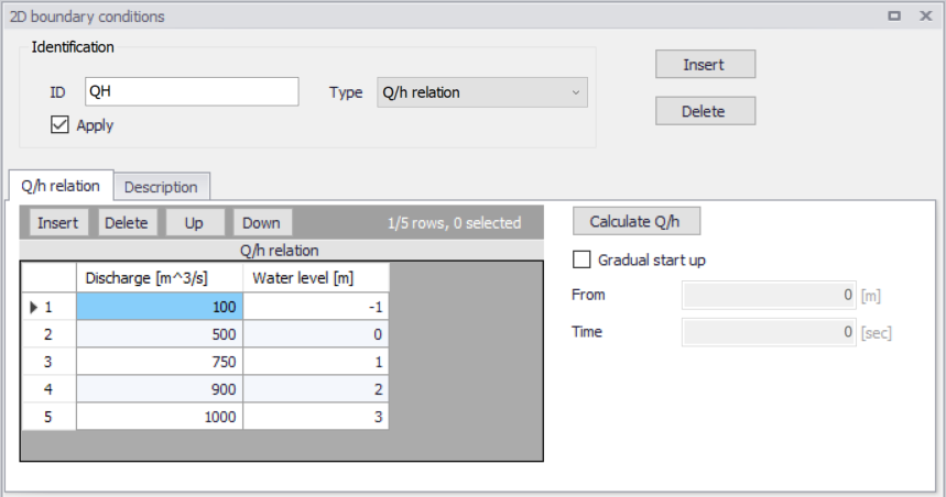
Figure: The rating curve secondary table on the Q/h Tab page on the 2D boundary conditions editor

Calculate Q/h

The Q/h relation rating curve may be automatically generated via the ‘Calculate Q/h’ button.

 

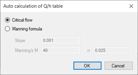
Figure: The dialog for configuring the auto-calculation of Q/h table values

The Q/h relation is computed using the topography in the mesh/grid along this boundary. Thus, topography values must have been interpolated for the mesh/grid prior the use of this tool.

 

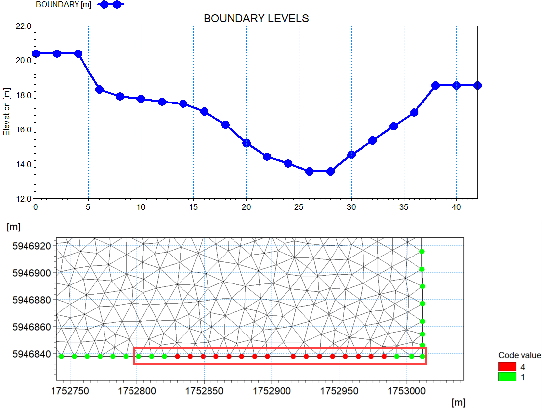
Figure: Illustration of topographical cross section (top) along an e.g. mesh boundary (bottom).

Discharge values are computed for various water levels, either using the ‘Critical Flow’ or the ‘Manning Formula’ as specified in the ‘Auto calculation of Q/h table’ dialog.

If the latter is chosen the bed slope and Manning’s "n" or "M" must be specified.

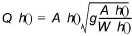
In case the critical flow formula is used, Q is calculated from:

 

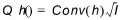
In case of uniform flow by Manning’s Formula, Q is calculated from:

 

Where:

= Level dependent discharge

= Level dependent area (from the cross section processed data)

= Level dependent width (from the cross section processed data)

= Bed slope

 = Level dependent conveyance calculated as a function of the resistance type defined for the cross section

 

Where:

 = Manning number defined in the 'Auto calculation of Q/h table' dialog

Gradual start up

A soft start option for applying the boundary condition is offered via the ‘Gradual start up’ option. One may specify a soft start interval during which boundary values are increased from a specified reference value to the specified boundary value to avoid shock waves in the model.

Free Outflow Boundaries

The free outflow condition is typically used at downstream boundaries where the water is flowing out of the model. This type of boundary does not require additional input in the editor.

Source Boundaries

Source boundaries are used to define local sources (or sinks) of water inland within the 2D domain (as opposed to along the domain perimeter).

Sources may be specified via the 2D Boundary Conditions editor by clicking on the ‘Insert’ button, or on the Map using the ‘Edit features’ toolbox on the 2D Overland menu ribbon or the Flooding layer editing tools toolbar. Point sources may be of type:

• Single point source
• Single distributed source
• Connected point source

 

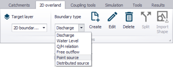
Figure: Adding Source boundaries on the Map using the Edit features toolbox on the 2D Overland menu ribbon

On the 2D Boundary Conditions editor, the 'Locaion' and 'Temporal Variation' for sources should be defined. The editor also has a Description tab for any notes about each source boundary item.

Location

Single point source

Define the x- and y-coordinates of the source on the Location tab page. You may also use the arrow button to graphically select a location on the Map. The x- and y-coordinates in the editor are updated accordingly.

 

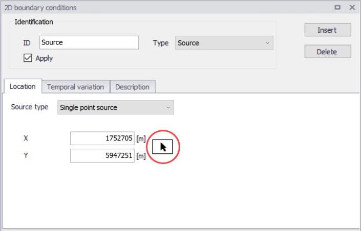
Figure: Locate the 2D point source graphically on the Map using the arrow button

Single distributed source

A distributed source is characterized by a polygon area in MIKE+. For this type of source, the specified discharge value is distributed (i.e. weighed distribution based on element area) in all mesh/grid elements within the polygon.

Define the x-and y-coordinates for the polygon in the secondary table on the Location tab. Alternatively, draw the distributed source polygon on the Map via the arrow button beside the secondary table.

The Edit Features toolbox on the 2D Overland menu ribbon, or the Flooding Layer Editing Tools map toolbar may also be used to create or edit distributed source polygons on the Map.

 

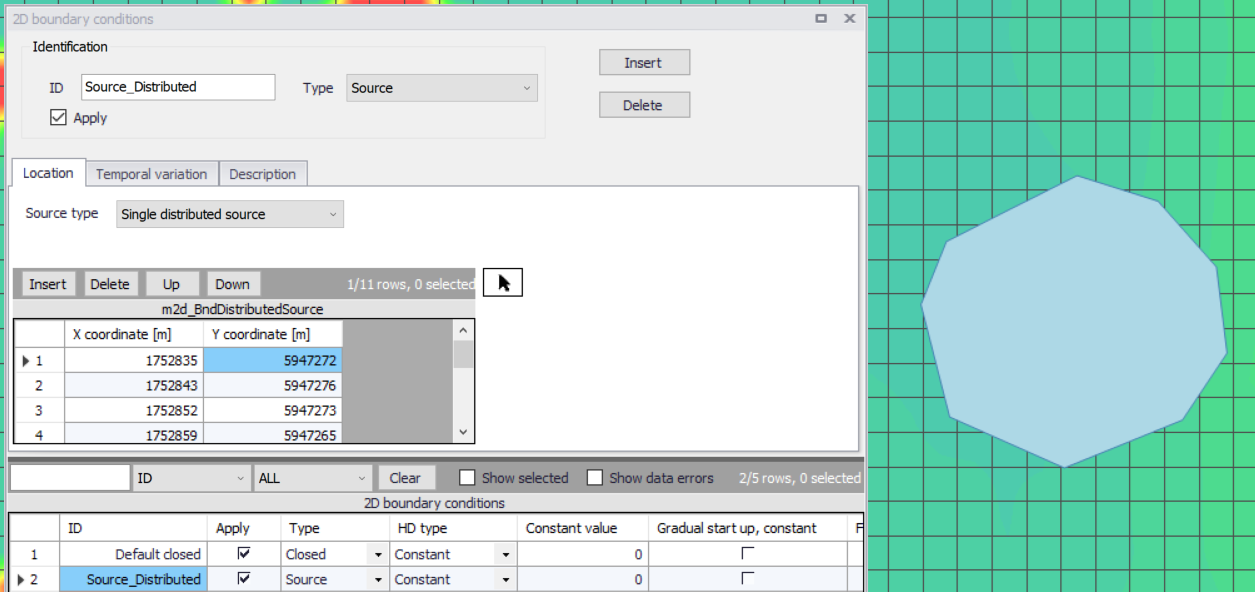
Figure: Distributed Source location on the 2D Boundary Conditions editor and the Map

If source velocity is applied (in the 'Temporal variation' tab), the specified velocity values are not distributed but remain identical in all mesh/grid elements within the polygon.

Connected point source

Connected sources are defined with two source locations (i.e. a sink and a source). For this option the source contribution to both the continuity equation and the momentum equations is taken into account.

Define the coordinates for the Sink and Source points on the Location tab. Alternatively, locate the points on the Map via the arrow buttons beside the input boxes.

The Edit Features toolbox on the 2D Overland menu ribbon may also be used to edit connected point source segments on the Map.

 

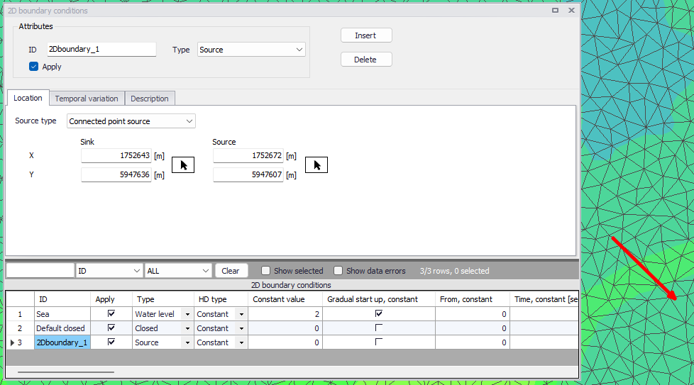
Figure: Define locations for the First Source and Second Source points for Connected Point Sources on the 2D Boundary Conditions editor and the Map

A positive discharge specified in the ‘Temporal Variation’ tab represents a flow pulled from the 2D domain at the Sink location, and reintroduced in the 2D domain at the Source location.

The velocity by which the water is discharged into the domain must be specified. Note that the contribution to the momentum equation is only taken into account when the water is discharged into the ambient water (i.e. the magnitude at the Second Source point is positive).

Temporal Variation

Define whether the source is defined as:

• Constant
• Varying in time
• Q/h relation

For time-varying sources, specify a timeseries file (*.DFS0) containing source information (i.e. discharge and velocity components, if needed). The data must cover the complete simulation period, but the time step may differ from the time step of the hydrodynamic simulation. A linear interpolation will be applied if the time steps differ.

For the Q/h relation type (not available for distributed sources), specify a time series files (*.dfs0) containing the relationship between discharge and water level. The file must use a relative item axis describing the water level (where the unit must be meter) and must contain a dynamic item describing the discharge.

 

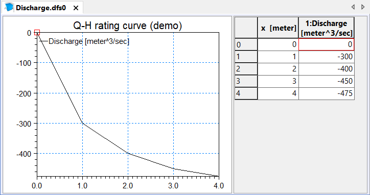
Figure: .dfs0 file containing a Q/h relation

Activate the ‘Apply source velocity’ if desired, for which the source contributions to the continuity equation as well as the momentum equation are both taken into account. In this case, the u- and v-velocity components need to be specified together with the source magnitude (i.e. Discharge). Otherwise, the source has no velocity component, for which only the source contribution to the continuity equation is considered. Note that connected point sources shall always have associated velocity components defined, and thus the ‘Apply source velocity’ option for these types of boundaries is disabled (for a Q/h relation type, these velocity components must be specified as a time series, using a regular time axis).

See the next section on 'Source Types' for more details.

 

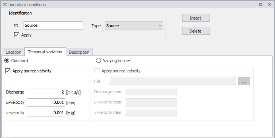
Figure: Temporal Variation tab for Source 2D boundary conditions

Source Types

For sources with no velocity component defined, only the source contribution to the continuity equation is taken into account. For this option, specify only the magnitude of the source. If the magnitude of the source is positive, water is discharged into the ambient water. If the magnitude is negative, water is discharged out of the ambient water.

For sources with velocity components defined, both the source contribution to the continuity equation and the momentum equations is taken into account. For this option, specify both the magnitude of the source and the velocity by which the water is discharged into the ambient water. Note that the contribution to the momentum equation is only taken into account when the magnitude of the source is positive (water is discharged into the ambient water).

Interpolation Types

For time-varying discharge and water level boundary types, the time step of the related timeseries data file does not need to match the hydrodynamic calculation time step. Thus, value interpolation may be required during computations. The interpolation method may be set as:

• Linear: Values obtained from a linear function (straight line) between 2 known value points.
• Piecewise cubic: Values obtained from a cubic polynomial approximation over sub-intervals.

In the cases with values varying along the boundary (i.e. Water level varying in domain and time), two methods of mapping from the input data file to the boundary section are available:

• Counter-clockwise definition: The first and last points of the line (i.e. *.DFS1) are mapped to the first and the last nodes along the boundary section, respectively, and the intermediate boundary values are found by linear interpolation.
• Clockwise definition: The last and first points of the line are mapped to the first and the last nodes along the boundary section, respectively, and the intermediate boundary values are found by linear interpolation.

Define these time- and space-wise interpolation settings in the Interpolation tab page of the 2D Boundary Conditions editor. These options are available for time-varying Discharge and Water Level boundaries.

These settings may also be modified for a 2D boundary condition under the ‘Interpolation type in time’ and ‘Spatial order along boundary’ columns in the overview table at the bottom of the editor.

 

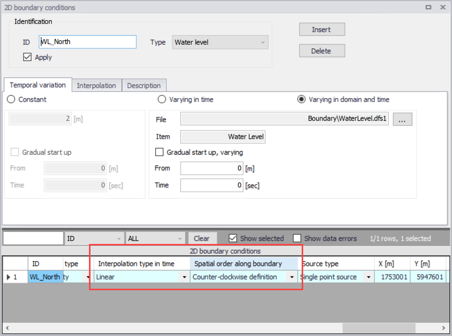
Figure: The ‘Interpolation type in time’ and ‘Spatial order along boundary’ attributes in the 2D boundary conditions overview table

Description

It is possible to provide a description of the boundary condition using the Description field.

An 'Event ID' may also be associated with the boundary condition. The purpose of the event ID is to automatically filter the boundary conditions to include in a given simulation by selecting the corresponding event ID during the simulation execution, i.e. in the 'Simulation setup' editor. When a boundary condition is associated with a specific event ID, it will only be used in simulation setups defined with this same ID. The value 'Default (any event)' indicates that the boundary condition is not associated with any specific event and will be used in all simulations. It is possible to either use the pre-existing IDs available in the list or to add or edit IDs using the '…' option at the bottom of the list. See the 'Simulation Setup' chapter for additional information.

Warning

2D boundary conditions other than sources can not overlap in space, even if they are associated with different events.