Update parameters
The 'Update parameters' editor is used for adding the measurement time series and defining their accompanying weighting functions. These definitions are the core of the data assimilation set up.
Measurements are added or deleted using the 'Insert' or 'Delete' buttons at the top of the editor. They can also be added, edited and deleted from the map, working with the 'DA update' target layer. A measurement's correction can be switched on and off using the 'Apply' option (so no need to delete measurements that are temporarily inactive).
Each measurement must have a specification of where in the network it is located, the type of the observed quantity and a time series with observed values, see the detailed description of the parameters below.
Note about water level update
In general measurements of water level (or depth) result in an indirect correction of the discharge. A discharge measurement (which causes injection/extraction of lateral flow) will have only little effect on the water level at the measurement location. If the simulated water level is important, level/depth measurements should be preferred over discharge measurements.
Note about time steps
While updating, DA corrects the simulation in every simulation time step. If the time stamps of the measurement series do not coincide with the simulation, the measurement values are interpolated linearly. The measurement time series may have non-equidistant time steps but be aware that interpolation will take place also over long periods of time, and that this may be misleading if the time gap is due to missing values.
Note about missing values
Missing values should be represented by delete values in the dfs0-file. Delete values in the measurement time series will trigger one of two behaviours
- If the weighting function does not include an error forecast model, the correction drops to zero while the observations are missing. This can cause abrupt changes in the correction, which might show as instabilities.
- If an error forecast model is specified, the error forecast will kick in while observations are missing, so updating in the period with missing data is based on a simulated error rather than on the observed error.
Measurement location
River ID: The name of the river where the observation point is located. It can be chosen from the list opened using the '…' button.
Chainage: Chainage along the river where the observed data is located. The chainage does not have to coincide with the location of a calculation point since DA interpolates the model state linearly between the two nearest grid points of the grid-point type, which relates to the type of the 'Updated item' (i.e. water level grid points for measurements of 'Water Level' / 'Water Depth' and discharge grid points for 'Discharge' measurements).
Updated item: The type of variable on which the update is performed. Depending on the modules included in the simulation (in the 'Model type' editor), the type can be either a water level, a water depth, a discharge or a WQ component.
WQ component: The component to be updated must be selected from the list of components defined for the Transport module.
File name: The time series file containing the observed data. The '…' button may be used to either browse, create or edit the time series.
Item ID: This field shows the name of the item selected in the time series. The type of the item must match the type specified in 'Updated item'.
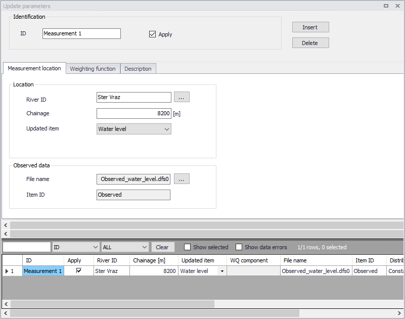
Figure: The Update parameters editor
Weighting function
A weighting function definition must be specified for each measurement with the main purpose of defining how model corrections at the measurement location are distributed to neighboring calculation points in the river network. . This can be viewed as "short-circuiting" the Kalman filter approach, as the weighting function is rooted in the user's estimate, not in the model's dynamics.
Distribution type
Three different types of distribution are available:
- Constant: in this case the error correction is distributed evenly over the grid points between the specified smallest and highest chainages.
- Triangular: in this case the error correction is linearly decreasing from a maximum correction at the measurement location (specified in the 'Measurement location' tab) to 0 at the smallest and highest chainages.
- Mixed exponential: in this case the error correction is decreasing according to an exponential function from a maximum correction at the measurement location to the smallest and highest chainages, where the correction is about 0.01 times the correction at the measurement location.
Amplitude
The amplitude specifies the fraction of the observed error at the measurement location that should be applied as error correction at that point. The amplitude should be in the range from zero to one. Theoretically, the amplitude reflects the confidence in the observation as compared to the model forecast. That is, if the amplitude equals one, the measurement is assumed to be perfect, whereas for smaller amplitudes, less emphasis is put on the measurement as compared to the model forecast. In practice, the amplitude works as an exponential smoothing, because even for low fractions the simulation will eventually approach the measurement, due to the correction taking place every simulation time step. An amplitude of one may result in an instability during the first time steps with updating, due to all of the error being corrected at once during the very first updating step. The destabilizing effect of a high amplitude can be counteracted by defining a 'Soft start' (see below).
Smallest chainage
It represents the start point along the river where the correction is applied (in the river where the measurement point is located). It corresponds to the upstream chainage for a river with a positive flow direction, or the downstream chainage for a river with a negative flow direction.
Highest chainage
It represents the end point where the correction is applied (in the branch where the measurement point is located). It corresponds to the downstream chainage for a river with a positive flow direction, or the upstream chainage for a river with a negative flow direction.
Include connected rivers
If this option is selected, the correction is also applied to tributaries (if any) which are connected to the main river between the specified smallest and highest chainages. The correction is applied within the same extent and with the same amplitude and distribution as for the river where the measurement is located.
Soft start
Number of time steps used to fade up the correction initially, starting from zero correction at the first updated time step up to full correction after the fade-up period. The fade-up follows a sine curve from trough to peak. A soft start helps avoiding model instabilities since the error correction value is introduced gradually rather than abruptly. This is especially relevant if the weighting function has an amplitude larger than around 0.25. An exact threshold cannot be given, as the dampening effect of a small amplitude also depends on the simulation time step.
Include error forecast
The correction up to 'Time of forecast' may be enhanced by error forecasting at updating points after Time of forecast'. This avoids discontinuities that would occur by stopping the correction abruptly at 'Time of forecast' and prolongs the effect of correction. It is mandatory and always included, when updating on discharge measurement. When active, an equation defining how the error evolves over time must be selected from the list of available equations. Initially the list of equations is empty, and at least one equation must be set up in the 'Error forecast equations' editor. Note that several measurements can use the same error forecast equation (also if the equation has estimated parameters).
Guidelines for defining the weighting function are:
Discharge measurements
Do not include downstream points in the update range, as a discharge correction downstream is not "visible" at the measurement's location. This can lead to overcompensation, when DA attempts to quantify the deviation between simulated and observed discharge. Good practice is to distribute the discharge correction over a few of the nearest upstream points. Distributing over a couple of points spreads out the correction a bit, thus reducing abrupt changes, but distributing the correction far upstream will cause an unwanted time-delay before the correction reaches the measurement location. This can lead to overcompensation as well. Do not 'Include connected rivers' for discharge measurements unless you specifically want to distribute a part of the correction flow to (the end) of a tributary.
The discharge correction is added as a lateral flow to water level points. A 100% correction of discharge can be obtained by defining a 'Constant' distribution with 'Amplitude' equal to one, and an update range that includes only the nearest upstream water level point.
Water level/depth measurements
It is common practice to define a 'Triangular' distribution. If the water level measurement is located in a pool behind a control structure, the update range should start at the upstream extent of the backwater and end at the measurement location. This will prevent the correction from "going across" the control structure.
In general, an update range should not include a control structure, because it is hard to estimate a meaningful shape of the weighting function 'by hand' on the far side of the control structure. Extra care must be taken when 'Include connected rivers' is on, if the tributaries contain control structures.
'Include connected rivers" can help to avoid the abrupt level changes that can be the result in the tributaries if only the main river is corrected. When 'Include connected rivers' is on, a distance calculator traverses the network behind the scenes and the distance from some point to the measurement location determines whether the point is inside the correction range. Be aware of loops in the network in the vicinity of measurements which 'Include connected rivers'. The loop might distance-wise be a short circuit, which creates a path to points downstream of the measurement point, which are inside the upstream range's correction scope.
Description
The description tab can store information describing the measurement location and its update parameters.