2D Numerical Settings
Configure 2D model numerical solution settings in the 2D Numerical Settings editor.
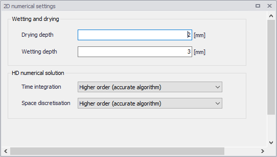
Figure: The 2D Numerical Settings editor
HD Numerical Solution
The 2D model simulation time and accuracy can be controlled by specifying the numerical scheme used in the calculations. Define the numerical solution technique to use in the 2D overland computations under the HD Numerical Solution section. Both the scheme for time integration and for space discretization can be specified:
- Lower order: First-order explicit Euler scheme. Faster but less accurate.
- Higher order: Two-stage explicit second-order Runge-Kutta scheme.
More details on the numerical solution techniques are presented in the MIKE 21 Flow Model FM Hydrodynamic and Transport Module Scientific Documentation.
If the important processes are dominated by convection (flow), then higher order space discretization should be chosen. If they are dominated by diffusion, the lower order space discretization can be sufficiently accurate. In general, the time integration and space discretization methods should be the same.
Choosing the higher order scheme for time integration will increase the computing time by a factor of 2 compared to the lower order scheme. Choosing the higher order scheme for space discretization will increase the computing time by a factor of 1½ to 2. Choosing both as higher order will increase the computing time by a factor of 3-4. However, the higher order scheme will in general produce results that are significantly more accurate than the lower order scheme.
Wetting and Drying
Moving boundaries (i.e. wetting and drying fronts) in 2D overland numerical computations are dealt with by reformulating the computational problem for small depths and removing elements/cells from the calculation when the depths are very small. This approach is based on work by Zhao et al. (1994) and Sleigh et al. (1998). The reformulation is made by setting the momentum fluxes to zero and only taking the mass fluxes into consideration.
The depth in each element/cell in the 2D domain is monitored against the following threshold values:
- Drying depth (\(h_{dry}\))
- Wetting depth (\(h_{wet}\))
During overland computations, the elements are classed as dry, partially dry or wet in comparison to these depth thresholds. Also, the element faces are monitored to identify flooded boundaries:
- An element face is defined as flooded when the water depth at one side of the face is less than \(h_{dry}\) and the water depth at the other side of the face is larger than \(h_{wet}\).
- An element is dry if the water depth is less than \(h_{dry}\) and none of the element faces are flooded boundaries. The element is removed from the calculation.
- An element is partially dry if the water depth is larger than \(h_{dry}\) and less than \(h_{wet}\), or when the depth is less than \(h_{dry}\) and one of the element faces is a flooded boundary. The momentum fluxes are set to zero and only the mass fluxes are calculated.
- An element is wet if the water depth is greater than \(h_{wet}\). Both the mass fluxes and the momentum fluxes are calculated.
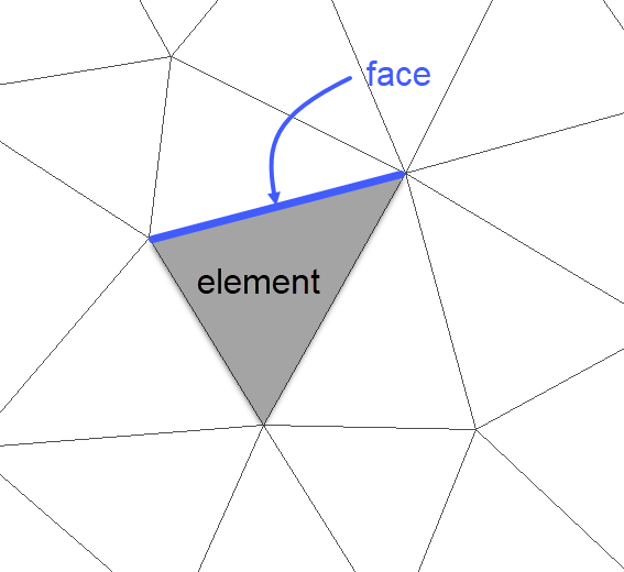
Figure: Illustration of elements and element faces
A non-physical flow across the face will be introduced for a flooded face when the surface elevation in the wet element on one side of the face is lower than the bed level in the partially wet element on the other side. To overcome this problem the face will be treated as a closed face.
In case the water depth becomes negative, the water depth is set to zero and the water is subtracted from the adjacent elements to maintain mass balance. In addition, the conserved variables \(h_{u}\) and \(h_{v}\) in the adjacent element where mass is subtracted, is corrected so that the velocities u and v remain the same. When mass is subtracted from the adjacent elements the water depth at these elements may become negative. Therefore an iterative correction of the water depth is applied (max 100 iterations).
Note on volume preservation
When an element is removed from the calculation, water is removed from the computational domain. However, the water depths at the elements, which are dried out, are saved and then reused when the element becomes flooded again.
Note on wetting and drying values
The wetting depth, \(h_{wet}\), must be larger than the drying depth, \(h_{dry}\).
The default values are: drying depth \(h_{dry}\) = 5 mm and wetting depth \(h_{wet}\) = 10 mm. For floodplain simulations, the values for wetting and drying depths should be relatively low to minimize water balance errors. A reduction factor of up to 5 is viable.
AD and MIKE ECO Lab Numerical Solution
Define the numerical solution technique to use in the Transport modules of the 2D overland simulations. The corresponding parameters become visible when the Advection-Dispersion or the MIKE ECO Lab modules are active in the project.
Both the scheme for time integration and for space discretization can be specified:
- Lower order: Faster but less accurate scheme.
- Higher order: Slower but more accurate scheme.
More details on the numerical solution techniques are presented in the MIKE 21 Flow Model FM Hydrodynamic and Transport Module Scientific Documentation.
The time integration of the transport (advection-dispersion) equations is performed using an explicit scheme. Due to the stability restriction using an explicit scheme the time step interval must be selected so that the CFL number is less than 1. A variable time step interval is used in the calculation and it is determined so that the CFL number is less than a critical CFL number in all computational nodes. To control the time step it is also possible for the user to specify a minimum time step and a maximum time step. The time step interval for the transport equations is synchronized to match the overall time step specified for the hydrodynamic simulation in the 'Simulation setup' editor.
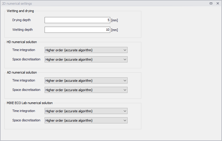
Figure: The numerical settings with Transport modules active