2D WQ Evaporation

The following sections describe the data requirements for the different ways of specifying 2D water quality characteristics for 2D evaporation boundaries in MIKE+.

The structure and data requirements for 2D evaporation boundaries are very similar to those for precipitation boundaries described in the previous section (see chapter 2D WQ Precipitation).

Also, note that it is usually most sensible to set the concentration of the evaporated water mass to zero, in which case the component is conserved in the water.

Ambient Concentration

For this type of 2D WQ evaporation input, the concentration of the evaporated water mass is set equal to the concentration of the ambient water in the domain.

Thus, this type of WQ boundary condition does not require additional details on evaporation concentrations.

Uniform

Use this option if evaporation boundary concentrations shall remain constant (in time and domain).

Under the Evaporation Concentration Details section define:

• Evaporation concentration value: Specified concentration of the selected/active pollutant component in the evaporation boundary condition.
• Soft start interval: Soft start interval during which WQ boundary values are increased from 0 to the specified value in order to avoid shock waves being generated in the computations.

Specify parameters for Uniform 2D WQ Evaporation conditions under the Evaporation Concentration Details section on the editor. A list of WQ components in the model setup is shown in the table overview at the bottom of the editor.

Varying in Time

The case with evaporation concentrations varying in time but constant in domain requires a (*.DFS0) data file containing timeseries data on concentrations (in component unit).

The data must cover the complete simulation period, but the time step of the input data file does not need to be the same as the time step of the hydrodynamic simulation. A linear interpolation will be applied if the time steps differ.

 

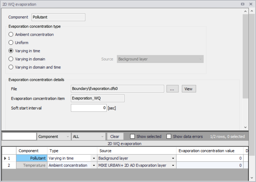
Figure: Data requirements for ‘2D WQ evaporation’ boundaries that are ‘Varying in time’

Varying in Domain

2D WQ evaporation boundary characteristics for various WQ components may also be modelled as varying in domain (constant in time). Input for this type of 2D WQ boundary may be defined using:

• MIKE+ 2D AD Evaporation layer
• Background layer

The data requirements for each are described in the following sections.

MIKE+ 2D AD evaporation layer

This option requires definition of ‘2D AD evaporation’ polygon features on the Map.

One may use the Edit Features toolbox from the 2D Overland menu ribbon, or the Flooding Layer Editing Tools toolbar on the Map. Use the ‘Create’ tool to draw features on the Map. Right-click to remove the last vertex added, and double-click to finish polygon drawing.

Under the ‘Evaporation Concentration Details’ section on the editor, define the 'Default evaporation concentration'. This value will be used over areas in the domain for which 2D AD evaporation parameters are not defined via the ‘2D AD evaporation’ polygons on the Map.

Records for 2D AD evaporation polygons drawn on the Map are listed in the table on the 2D WQ Evaporation editor. New records cannot be added from the tabular view. They are only added when drawing a new polygon on the map.

 

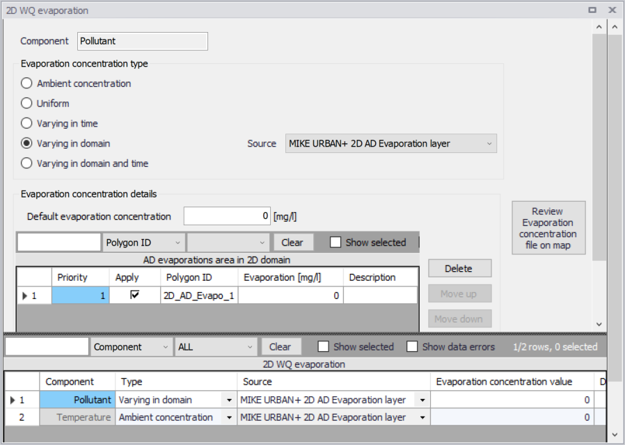
Figure: Edit the properties of the ‘2D AD evaporation’ layer polygons in the table on the 2D WQ Evaporation editor

Specify the concentration value (related to the active/selected WQ component) for each polygon feature on the table. All items from the table are WQ component-specific. The table has the following columns:

• Priority: This is equivalent to the row number. Indicates the order with which values for overlapping features will be prioritized for use in the model.
• Apply: Check box allowing activation/deactivation of individual polygon features without deleting the polygon and its properties from the Map.
• Polygon ID: This is a text string used to identify the polygon.
• Evaporation: This is a numerical field containing the evaporation concentration value assigned to the polygon. The unit is shown in the header (same unit as for the numerical field above the table).
• Description: This is an optional text string used to save a free user description for a polygon feature.

Use the ‘Review evaporation concentration file on map’ button to generate a 2D file from the evaporation concentration configuration and view the generated file on the Map. The generated 2D file type depends on the defined 2D model type: *.DFS2 grid files for rectangular grid models, and *.DFSU unstructured files for flexible mesh models.

When the file is created, it is then added as a layer on the Map (i.e. it is listed in the tree view and visible on the Map). When the file contains multiple items/components, the component which is drawn on the map is the active component in the overview table. If the file was already loaded as a layer, it is only refreshed (with new data, and with the last active component number).

Background layer

This option requires specification of a background polygon layer to represent domain-varying 2D evaporation concentrations.

The ‘Evaporation concentration details’ section on the 2D WQ Evaporation editor displays:

• Default evaporation concentration: This value will be used over areas in the domain for which parameters are not defined with the background layer polygons.
• Layer: A drop-down list populated with valid layers loaded as background layers on the Map. A layer is valid if it is a *.TAB, or *.SHP polygon layer.
• Evaporation concentration item: Drop-down list populated with the full list of attributes from the selected layer.
• Unit: Drop-down list showing unit options depending on the 'Type' of WQ component as specified in the 'WQ components' editor:
  • For Type = 'Pollutant', it shows the list of all supported units for concentration (e.g. mg/l, g/m³, kg/m³, g/l, μg/l, pound/(feet US)³, pound/feet³, pound/(yard US)³, pound/yard³, etc.)
  • For Type = 'Microorganism', it shows the list of all supported units for bacteria / micro-organism concentrations (e.g. million/100 ml, per 100 ml, per liter, etc.)
  • For Type = 'Temperature', it shows the list of all supported units for temperature (e.g. degree Celsius, degree Fahrenheit, degree kelvin, etc.)
  • For Type = 'pH', it shows a single undefined unit [].
  • For Type = 'Salinity', it shows the list of all supported units for salinity (e.g. PSU, per thousand, etc.)
  • For types 'Water age' and 'Water blend', it shows a single undefined unit [].
• Soft start interval: Interval during which WQ boundary values are increased from 0 to the specified value in order to avoid shock waves in the computations.

The ‘Review evaporation concentration file on map’ button generates a 2D file from the evaporation concentration configuration and loads the generated file on the Map. The generated 2D file type depends on the defined 2D model type: *.DFS2 grid files for rectangular grid models, and *.DFSU unstructured files for flexible mesh models.

When the file is created, it is then added as a layer on the Map (i.e. it is listed in the tree view and visible on the Map). When the file contains multiple items/components, the component which is drawn on the map is the active component in the overview table. If the file was already loaded as a layer, it is only refreshed (with new data, and with the last active component number).

Varying in Domain and Time

The case with evaporation concentrations varying both in time and domain requires a 2D file with concentration values. The file must be a 2D unstructured data file (*.DFSU) or a 2D grid data file (*.DFS2) with ‘Dimensionless Factor ()’ Item type.

The area in the 2D data file must cover the model domain. If a *.DFSU file is defined, piecewise constant interpolation is used to map the data to the domain mesh. If a *.DFS2 file is defined, bilinear interpolation is used to map the data to the domain grid.

The data must cover the complete simulation period, although the time step of the input data file does not have to be the same as the time step of the hydrodynamic simulation. A linear interpolation will be applied if the time steps differ.

On the editor, define the 2D data file under the ‘Evaporation Concentration Details’ section:

• File: A drop-down list of valid 2D layer files on the Map. A file is valid if it is a time-varying *.DFS2 or *.DFSU file with Item type = 'Dimensionless Factor'. The ellipsis button launches the 'Open a dfs file' dialog that is used to locate a valid time-varying 2D file. The dialog filters on types '2D Grid file (*.DFS2)' or 'Unstructured data file (*.DFSU)', and has a drop-down list for Items that may be loaded. The 'View' button opens the selected time-varying 2D file for viewing/editing. It launches the Grid Editor if a *.DFS2 file has been selected in the editor. If a *.DFSU file has been selected, it opens the file using the Data Manager.
• Evaporation concentration item: Non-editable text box displaying the selected Item from the loaded file. The database stores one file name and item for each WQ component.
• Soft start interval: Interval during which WQ boundary values are increased from 0 to the specified value in order to avoid shock waves in the computations.