Curves and Relations
In the 'Curves and Relations' editor, a number of tabular data used in other data dialogs are specified. Available tabular data types vary depending on the project model type.
The Curves and Relations editor organizes the related input data into the following groups:
- Identification: General identification and curve type information
- Curve Values: Secondary table containing tabular data values
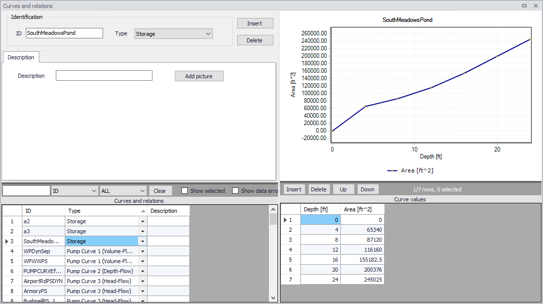
Figure: The Curves and Relations editor
Use the 'Insert' or 'Delete' buttons to add or remove records from the editor, respectively. Records are added to the primary table on the lower left corner of the editor.
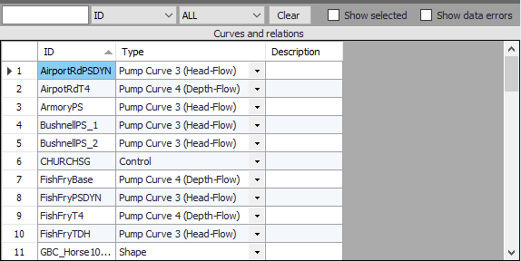
Figure: Primary table with the Curves and Relations list on the lower left side corner
Identification and Description
The identification groupbox holds curve ID and Type information.
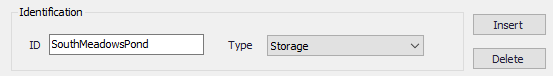
Figure: The Identification groupbox
Add optional descriptive information for a curve in the Description tab. An option for adding an images is also available.
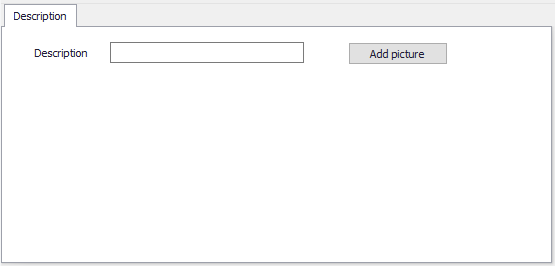
Figure: The Description tab
| Edit field | Description | Used or required by simulations | Field name in datastructure |
|---|---|---|---|
| ID | Curve ID | Yes | MUID |
| Type | Type of curve | Yes | TypeNo |
| Description | User's descriptive information on the curve | No | Description |
Table: Edit fields in the Curves and Relations Identification and Description group boxes
Curve Values
After inserting a new curve, define the corresponding data values under the 'Curve values table' (i.e. secondary table in the lower right corner). Columns that should be filled vary depending on the curve and relation type.
A plot of the tabular data is also shown on the upper right corner of the editor.
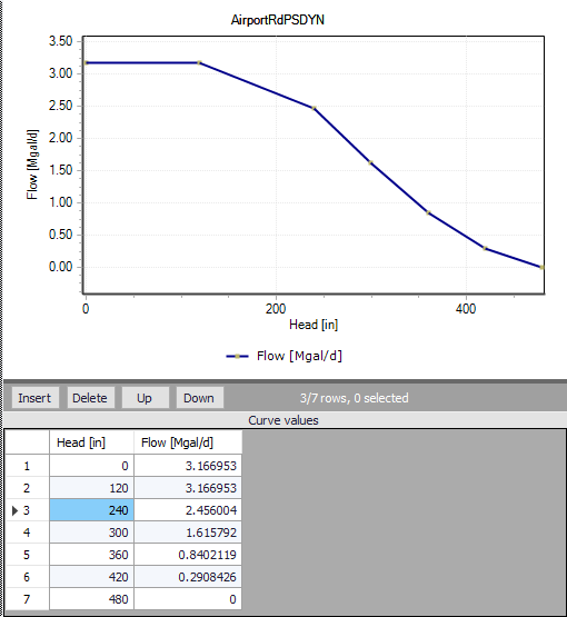
Figure: Secondary table containing Curves Values on the lower right corner, and corresponding plot
| Edit field | Description | Used or required by simulations | Field name in datastructure |
|---|---|---|---|
| ‘Value1’ | Value1, dependent on Type of curve (Depth, Inflow, Hour, Volume, Head) | Yes | Value1 |
| ‘Value2’ | Value2, dependent on Type of curve (Area, Outflow, Stage, Flow) | Yes | Value2 |
Table: Edit fields in the Curve Values secondary table
Warning
There are three pre-defined Time-Area Curves available by default (TACurve1, TACurve2 and TACurve3). These are used by default for catchments modelling, and should not be deleted, unless no catchments are about to use these curves.
Details for the different curve types
Capacity curves QH / QdH
It is possible to define two types of capacity curves in MIKE+; both are used to define pump operation.
The capacity curve can be a 'Capacity Curve QH' relation (for screw pumps) or 'Capacity Curve QdH' relation (for differential head pumps).
‘H' is the absolute water level in the pump's wet well (i.e. From Node), and 'dH' is the water level difference between the (downstream) 'To Node' and (upstream) 'From Node' locations.
If an offset is specified, this will be added to the capacity curve relation.
Also note that one may specify a pump capacity curve with energy consumption (i.e. Capacity Curve QdH & Power).
Pump acceleration curve
Pumps may be controlled by control rules. For PID-controlled pumps, the acceleration of a pump can be specified as dependent on the actual flow. This pump acceleration curve is then specified as a number of ‘dQ, dQ/dt’ values.
Regulation curves Qmax(H) and Qmax(dH)
The regulation curves Qmax(H) and Qmax(dH) are used in the regulation of the maximum discharge in links. The regulation can either be a maximum discharge as a function of the water level in a user-specified node, or a maximum discharge as a function of the water level difference between two user-specified nodes.
QH relation
QH relations can be used for outlets. Using a QH relation in an outlet means that you specify the discharge out of the outlet based on the water level in the outlet.
Valve rating curve
A valve is a functional relation between two nodes of a sewer network. The valve rating curve specifies the relationship between the valve opening (%) and resistance (k).
Time-Area curve
The Time-Area curve is used in the Time-Area runoff model. A Time-Area curve represents the percentage contributing part of the catchment surface as a function of time.
MIKE+ comes with three default Time-Area curves - TACurve1, TACurve2 and TACurve3 - applicable for rectangular, divergent and convergent catchments, respectively.
One can define other Time-Area curves. Each Time-Area value table must start with a pair of values (0,0) and must end with a pair of values representing the whole catchment contribution. MIKE+ maintains T-A curves in percent (%), and the last pair of values in the table must be (100,100).
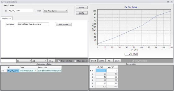
Figure: Example of user-defined Time-Area curve
Removal efficiency
There are three methods available for the removal of sediments in weirs. In one of these methods you specify the relation between discharge towards the weir and the removal efficiency, i.e. the efficiency curve. The removal efficiency is hence a function of Q and the efficiency (dimensionless 1/1).
Curb inlet DQ and QQ relations
Two curve types can be specified for two different types of Curb Inlets:
- DQ Relation (depth-discharge relation specified in the Curb Inlets dialog)
- QQ Relation (Qapproach-Qcapture relation specified in the On Grade Captures editor).
The DQ relation specifies the depth-based capacity curve for a SAG Type Curb Inlet. Values must be monotonously increasing in depth and discharge and starting at (0,0). For depths in excess of the maximum value specified in the last row of the table, the last corresponding discharge value is used.
The QQ relation specifies the relationship between approach flow in the overland flow network (Qapp) and the captured flow at the connection node for an On Grade Type Curb Inlet (Qcap). Values must be monotonously increasing and starting at (0,0). For approach discharges in excess of the maximum value specified in the last row of the table, the last corresponding capture discharge value is used.
Capacity curve QdH & Power
If specific power consumption in relation to pump levels is known, it is possible to include this in the model using the ‘Capacity Curve QdH & Power’ curve type.
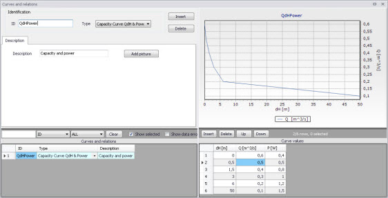
Figure: Pump capacity curve including power consumption
After the simulation with a ‘Capacity Curve QdH & Power’ the summary will contain information on the power consumption during the simulation period.
Runoff pollutants
This type of table is used in surface water quality (SWQ) boundary conditions as a way to define the Temporal Variation of surface stormwater loads as well as RDI stormwater loads.
The table serves as a lookup table for the boundary condition, where corresponding concentration values are determined based on runoff intensity. The tabular data set shall contain values for runoff intensity (i.e. the runoff divided by the total catchment area) and corresponding concentrations.
Basin geometry
Basin geometries are tabulated area-elevation functions. One specifies values for the parameters H, Ac, and As.
Ac is the cross-section area perpendicular to the main flow direction in the basin, which is used to calculate the velocity. As is the surface area of the basin (used to calculate the volume). Both parameters are specified as functions of the water level, H, in the basin.
The H-column for the basin geometry can start at any value, e.g. 0 for interpretation of H as depth in the basin. MIKE+ associates the first H-value to the bottom level of the node. This means that the same geometry can be reused in several places in the model.
The maximum level before flooding at a basin is either the highest H value of the geometry or the ground level. If the top of the basin geometry is below the ground level, the specified basin geometry is extended with additional points to allow for flooding.
The plot for 'Basin geometry' tables shows two types of points:
- Volume points: These are the raw points at levels H specified in the input table.
- Volume: These are extra points added at regular intervals between levels H specified in the input table. These extra points help better representing the actual variation of volume between input levels, which is not necessarily linear.
Generic control rule
Generic control rule tables are used for actions’ set point in control rules. They are lookup tables defining the functional relation between an actual input value (e.g. sensor reading or difference between sensor readings, etc.) and the set point value (or setting). The tabulated values are linearly interpolated between defined relations.
Control rule time series
Control rule time series tables are used for action’s set point in control rules. They are lookup tables explicitly defining the set-point value (or setting) for particular time periods (i.e. date/time). The tabulated values are linearly interpolated between defined values.
Crest level profile
The Crest level profile table is a Chainage-Level relationship describing embankment elevation profiles along rivers. It is used in defining lateral river bank and natural channel couplings. See '1D-2D Couplings' editor, 'Attributes' tab, for use of this curve type.
Depth dependent infiltration
This is a lookup table of Infiltration Rate and Depth values, used in 2D overland models. It is the Infiltration Curve input when 2D Infiltration is defined as ‘Varying in domain and flow dependent’ in the '2D Infiltration' editor.
Depth dependent Manning (M) or (n)
This is a lookup table comprised or Depth-Manning M (or Depth-Manning n) value pairs, used in 2D overland models. Used as Roughness Curve input when 2D Surface Roughness is defined as ‘Varying in domain and flow dependent’ and as a function of Depth in the '2D Surface Roughness' editor.
Flux dependent Manning (M) or (n)
This is a lookup data comprised or Flux-Manning M (or Flux-Manning n) value pairs, used in 2D overland models. Used as Roughness Curve input when 2D Surface Roughness is defined as ‘Varying in domain and flow dependent’ and as a function on Flux in the '2D Surface Roughness' editor.
Undefined type
The Undefined table type is an extra generic type of table which is only expected to be used in the rare case where none of the other specific table types are valid.