2D Eddy Viscosity
The eddy viscosity can be specified in one of four different ways:
- None
- Uniform
- Varying in Domain
- Smagorinsky Formulation
None
The eddy viscosity terms are omitted from the calculations.
Uniform
A constant eddy viscosity value in \(\text{m}^{2}/\text{s}\) is specified that applies to the entire 2D domain.
Varying in Domain
To define spatially varying 2D eddy viscosity, the following two sources of information can be used:
- MIKE+ 2D Eddy Viscosity Layer
- 2D File.
MIKE 2D eddy viscosity layer
MIKE+ 2D Eddy Viscosity Layer
This option enables an eddy viscosity layer to be graphically defined in the "Map" view using the tools available in the "2D overland" ribbon.
Steps to define eddy viscosity layers:
- Select the Target layer as "2D eddy viscosity"
- Click on "Create" and define polygons. Utilise the various editing tools to refine the polygons if necessary. Tip: specify a default eddy viscosity value in the 2D eddy viscosity table to automatically populate the values of a polygon as soon as it is digitised.
- In the 2D eddy viscosity table, the digitised polygons will be listed. Specify the eddy viscosity values for each of these polygons, and prioritise them using the up and down buttons (important if there are overlaps)
- Where the model domain is not covered by the roughness polygons the default value will be used in this area.
Clicking on "Review eddy viscosity file on map" will build a 2D eddy viscosity *.DFS2 file and add the layer to the map. This layer will also be saved in your project directory for use in the simulation. This file will also be created when starting the simulation, if it doesn't exist in the project directory of if input data have been modified.
2D File
Use a previously defined *.DFS2 or *.DFSU file with "Viscosity" item type as the 2D eddy viscosity.
Smagorinsky Formulation
Dynamically calculate eddy viscosity by means of the Smagorinsky formula.
A minimum and maximum value (\(\text{m}^{2}/\text{s}\)) for the eddy viscosity needs to be specified, along with either a uniform or spatially varying Smagorinsky coefficient. In the case of a spatially varying coefficient, a previously defined |\*.DFS2 or \*.DFSU file with "Dimensionless factor" item type can be selected.
Scientific Description
The effective shear stresses in the momentum equations contain momentum fluxes due to turbulence, vertical integration and sub-grid scale fluctuations. The terms are included using an eddy viscosity formulation to provide damping of short-wave length oscillations and to represent sub-grid scale effects (see e.g. Madsen et al., 1988; Wang, 1990).
The eddy coefficient, E, must fulfil the criterion:
(3.9) 
where l is a characteristic grid/element length (e.g. dx) and Dt the time step.
For the Smagorinsky formulation, Smagorinsky (1963) proposed to express sub-grid scale transports by an effective eddy viscosity related to a characteristic length scale. The sub-grid scale eddy viscosity in the horizontal direction is given by
(3.10) 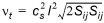
where \(c_{s}\) is a constant, l is a characteristic length and the deformation rate is given by
(3.11) 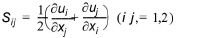
For more details on this formulation, the reader is referred to Lilly (1967), Leonard (1974), Aupoix (1984), and Horiuti (1987).
Recommended Values
The Smagorinsky coefficient, \(c_{S}\), should be chosen in the interval of 0.25 to 1.0.
Remarks and Hints
In the same way as for the bed resistance you can use the eddy coefficients to damp out numerical instability. This method should only be used as a last resort to your stability problem: The schematisation of the bathymetry and the boundary conditions are usually the primary causes for a model blow-up.
When you use the Smagorinsky formulation the CPU time for a simulation is increased.