Editing Tools

MIKE+ is very flexible in how a network or 2D overland model can be developed. Raw data can be brought into the model using a variety of input methods such as importing the data from a range of supported formats (see chapter Import and Export), utilising a range of tools available within the interface (e.g. chapter Interpolation and Assignment Tool), direct data entry into the MIKE+ tables or by visually digitising the data on the Map.

Overview

Graphical editing tools are available for all feature types such as:

• Model network elements (e.g. junction nodes, pipes, sewer manholes, storage tanks, pumps, valves),
• Demand points (consumption points),
• Load allocation points, or
• Catchments

Within each MIKE+ database table, functionality exists to efficiently edit the attributes of each model component.

Any alterations or changes made are immediately visible on the map and are automatically applied to the database tables. As each individual edit or update is recorded within a session, unlimited Undo and Redo is available, as long as the application is not closed.

 

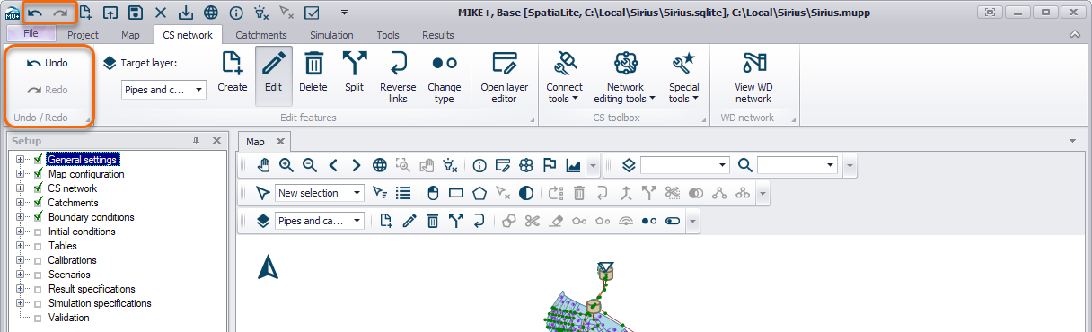
Figure: MIKE+ Graphical user interface with unlimited Undo and Redo functions

Graphical Editing

The easiest way of spatially defining a collection system or water distribution network, especially for smaller network additions to a model, is to graphically digitise the elements through the Map view.

To display the Map view, select Project | Map view. The Map view opens a drawing surface using the default coordinate system as defined during the creation of the MIKE+ project.

By utilising background maps (aerial photos, terrain, cadastral, asset layers, etc.) loaded into the Map view, components of a model can easily be graphically constructed.

Toolbars

Graphical editing tools, available both in the ribbon (e.g. in the CS/WD Network tab) or in the map view toolbar are used for interactively defining components of the model setup.

First a "Target Layer" must be selected. The list of target layers available in the map toolbar depends on the active modules in the project. The two figures below show the graphical editing tool bars for collection systems and water distribution systems respectively.

 

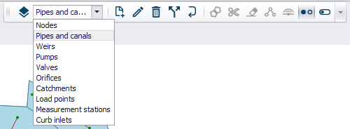
Figure: Collection System Network editing tools - Map view

 

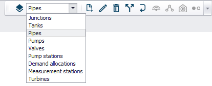
Figure: Water Distribution Network editing tools - Map view

After selecting a Target layer, the editing tools are available, and the required tool can be activated by clicking on the icon. The tool remains active until the icon is clicked again. Depending on the individual tool, a number of mouse-click actions are available within the Map view. Generally, single left mouse clicks will define extents, double clicks will complete the action, "enter" will finalise an action and "escape" will abort the tool.

A list of editing tools with a short description is summarised below.

 

Create new features

This tool activates the ability to add a new network component, depending on the component type (target layer) selection.

Points (e.g. Nodes/Junctions) are added using a single mouse click on the map view. If the mouse click occurs over an existing pipe, the symbol for a new node will appear on the pipe and you will be asked if you would like to split the pipe. "Yes" will create a new node and split the existing pipe in two, automatically connecting the node and pipes. "No" will create a node but not split the existing pipe, therefore the node will not be automatically connected to the network.

Other network components that are represented by a line (pipes, weirs, valves, etc.) require a single mouse click to start the digitisation. If the first click occurs over an existing point feature, a line feature will automatically be connected to this point. The line feature can continue being digitised using single clicks but a double mouse click is required to complete the line. If the double click occurs over a point feature, the network component will automatically be connected to this node. If the double click does not occur over a point feature, a new node/junction will automatically be created.

New polygon features (catchments) are defined with single mouse clicks on the map view to define the polygon shape and a double click (or click "enter") to complete the polygon.

If the digitisation of a new feature needs to be aborted partway through, click the Esc button on your keyboard or click on the "create new feature" button in the MIKE+ interface again to deactivate the tool.

 

Edit features

This tool is used to alter the geometry of an existing feature within the Map view. Click on the tool to activate it and then click on the network element to be changed. For point elements, it's location can be shifted. Shapes or lines (e.g. catchments or pipes) can be moved after clicking on the grab icon in the middle of the element. It is also possible to move the points defining a catchment or a pipe and therefore resize or rotate them.

 

Delete features

This tool is used to delete components within the Map view. Firstly, activate the tool by clicking on the icon. As you move around the visible network in the Map view, the cursor will change to + over an element that can be deleted, based on the selected target layer. Click on the element to delete it. Remember, it is possible to undo a deletion if something is deleted by mistake.

 

Split

This tool is used to graphically split a feature. To split a pipe, select the tool and click on the location of where the pipe is to be split. The tool automatically inserts a node at the split location. To split a catchment, draw a line across the catchment shape by a single click to start and a double click to complete the line (start and end must be outside the catchment boundary). The tool automatically deletes the existing catchment record and inserts two new catchment records. To split a river or 1D-2D coupling line, click on the location where the line should be split and the part of the line between the two closest vertices in both directions will be removed.

 

Reverse orientation of a line

This tool is used to swap the orientation of a line feature (from and to nodes/junctions) by clicking on the pipe. It is not possible to visually view the changes unless the pipe symbology has directional arrows included. The "From" and "To" node/junction change will be visible in the database tables.

 

Change element type

This tool is used to replace the type of point or line element, dependent on the selected target layer. A pipe can be replaced by a weir, pump, valve or orifice. A manhole can be replaced with a basin, outlet and junction.

 

Open/Close element

This tool is used to open or close a pipe within the network. Closing and opening actions alternate with every click. There is no visual change in the pipe appearance unless a dedicated symbology is used, but the underlying property "Enabled" will change and can be checked in the network tables. This tool is only available in Collection system mode.

 

Append catchment

This tool is used to insert a new catchment graphically by appending it to the external boundaries of existing catchments. Digitising the new catchment must start and end within an existing catchment. The face of the new catchment will automatically align with the existing catchments

 

Clip catchment

This tool is used to clip existing catchments defined by a polygon shape, excluding the remainder of the catchment. Activate the tool to draw a polygon (clipping extent). This can span over one or more catchments. Single mouse clicks will define the polygon and a double click will complete the polygon. To finalise the clip, press Enter on your keyboard and then the underlying catchment/s will be clipped, maintaining the same attributes as the original catchments except for the geometrical area.

 

Erase catchment

This tool is used to define an area of a catchment to be removed from an existing catchment (opposite of the clip tool). Single clicks will digitise the extent of the polygon to be removed, a double click will complete the polygon and once Enter is pressed on the keyboard, a polygon will be deleted from the existing catchments.

 

Connect catchment

Once a catchment is selected, this tool is used to connect the selected catchment to a node or a link by simply activating the tool and clicking on a node or link. If a node is selected, a new catchment connection will be created, appearing visually on the map and as a new row in the catchment connections table. It is important to note that a catchment can be connected to multiple nodes. If a link is chosen to connect the catchment, the chainages of the link to distribute the catchment load will be requested. For catchments distributed to multiple nodes and links, the proportion of rainfall runoff and population equivalent from the catchment going to the node/link must be defined.

 

Connect Pump Station (only in WD network)

This tool is used to connect a pump station to the water distribution network.

 

Connect Demand Allocation (WD)/Connect load (CS)

This tool is used to connect either a demand allocation or a load point to the network.

 

Connect Station (both CS and WD)

This tool is used to connect a measurement station to the network.

In addition to using the editing tools described above that allow you to work on an individual network element or define your network layout, there are several bulk editing tools associated with the selection toolbar. These tools, such as "Delete", union of pipes, etc will be executed on all selected network elements (see Selection).

Graphical Editing Step-by-Step Example (CS)

Select the ‘Rivers, collection system and overland flows’ mode (Project Model, from the main ribbon at the top of the MIKE+ interface). Make sure that all the modules you will need are turned on (from the ‘Setup’ tab on the left tree view, go to General Settings Model type, and select the required modules for the ‘Rivers, collection system and overland flows’ mode). E.g. if you will have catchments, make sure that the "Rainfall-runoff (RR)" module is ticked on.

The main components of a sewer network can be defined as points (manholes), lines (pipes, weirs, etc) and polygons (catchments). Either in the Map view (Project, Map view) or in the CS Network and Catchments ribbons, graphical editing tools are available. First, select the "Target layer" from the drop-down list and the available tools for the selected target layer will be visible (see figure below).

 

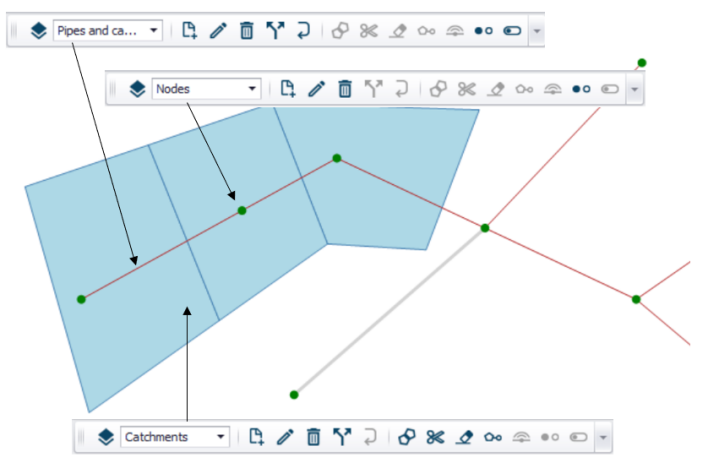
Figure: Tools activated for different "Target layers" (pipes, nodes, catchments)

To create new network components and add them to the model, first select the appropriate target layer, such as Nodes. The target layer selection will enable an appropriate set of tools.

 

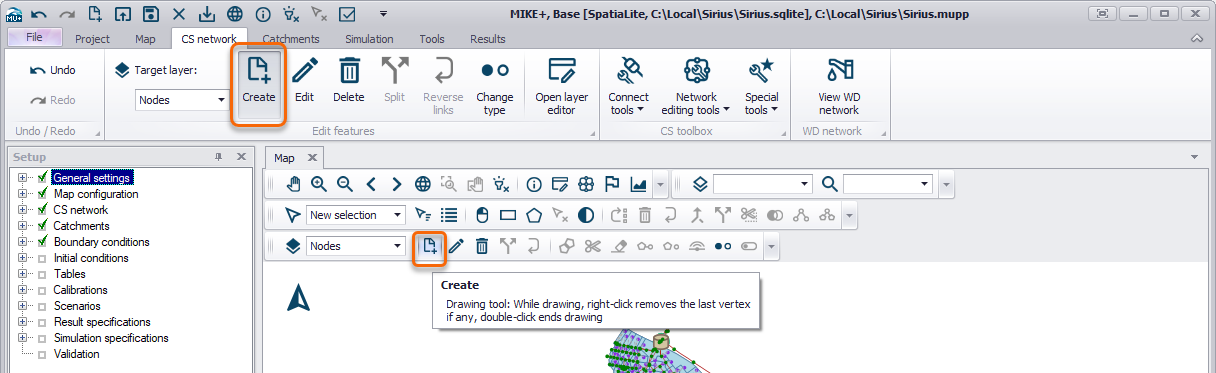
Figure: Use the Create tool to digitise nodes (manholes) for the collection systems network

Click on the Create tool from the network editing ribbon or floating toolbar, as shown in the figure above. The icon will become active (it will appear pressed down) and you can point and click within the Map window to graphically add manhole locations. When finished, click the Create tool again (it will pop back up) to deactivate the tool.

When adding nodes, you can change the type of node you want to create. For sewer networks, nodes can be manholes, basins, outlets or soakaways (figure above).

 

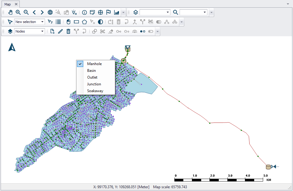
Figure: Right-click while in the node create mode will prompt you to select what type of node you want to create

To digitise links, select the Pipes and Canals layer from the Target Layer drop down list and click within the Map view to graphically add links using single mouse clicks to define the link and a double mouse click to complete a link. Continue digitising links while the tool is active. Tip: use the Esc button on the keyboard to keep the tool active but start digitising in a different area of the model. Note that the cursor changes to a circle when snapping onto existing nodes. If no node exists at the completion of a pipe digitisation, a new node will be created. To finish, click on the Create tool again to deactivate it.

 

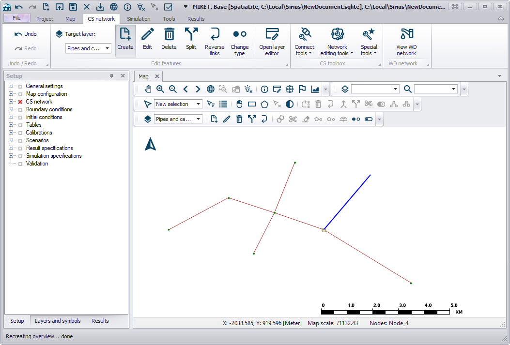
Figure: Use the Create tool for interactively laying out the network pipes in the CS mode

Catchments are defined as polygons. Digitise the polygon by clicking around the catchment extent to close a shape. Double-click to complete the catchment. To add an adjacent catchment without gaps or overlaps, activate the append polygon tool and then start the new catchment within the existing catchment, digitise the outer boundary (there is no need to digitise along the shared boundary) and then double click back in the existing catchment to complete. A new catchment will be created with the shared face between catchments exactly in line with each other, as shown in the Figure 8.8.

 

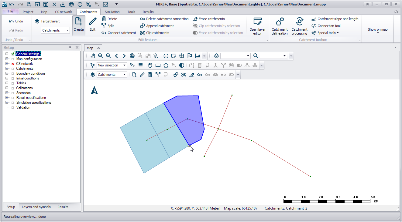
Figure: Graphically appended catchments

To graphically digitise water distribution network components, activate the water distribution mode by selecting Project Model Water Distribution from the main ribbon. The process of graphically adding pipes, junctions or any other network elements is the same as described above for the collection system described above.

Using the Editors

Once components of a model have been graphically digitised or imported into the model, there is often a need to edit the attributes of an element. This can be done by manually typing attribute data into the Editors or by utilising MIKE+ selection tools (Refer to chapter Map Menu) and table editing tools to edit the data en masse.

Identify the Location to Edit

A number of different methods exist to locate the attributes of the model to be edited.

MIKE+ has automatic data validation where missing or incorrect attributes are highlighted in orange. Model components where the data validation has identified issues can be summarised by ticking on "Show data errors" as shown in the figure below.

 

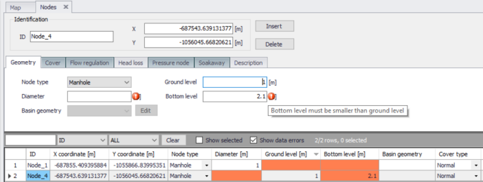
Figure: Show data errors

As the Map view is synchronised with the tables, locations can be selected in the Map view and the row corresponding to the highlighted element will be highlighted in blue in the table. Conversely, rows selected in the table will be highlighted in the Map view to visualise the locations.

Selected rows can be visualised together by ticking on "Show selected" as shown in the figure below.

 

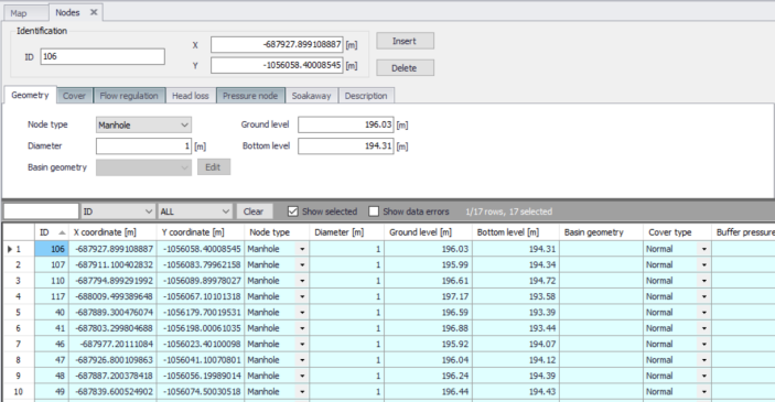
Figure: Summarise the selected rows by ticking on "Show selected"

A left mouse click on a table heading sorts the data (ascending to descending and vice versa). So outlying values can easily be identified, or a particular value can be found more efficiently.

Filters exist to sort by a table heading, a type of model component (e.g. manhole, basin, outlet or soakaway) or filter by typing part or all of the ID.

 

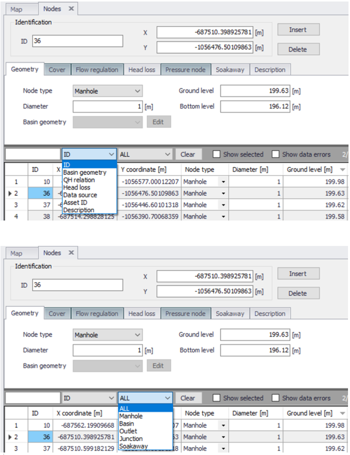
Figure: Filtering by header or model component type

A right click on a table heading opens the possibility to select by column, or select by attribute. Refer to chapter Map Menu for more on selecting by attribute.

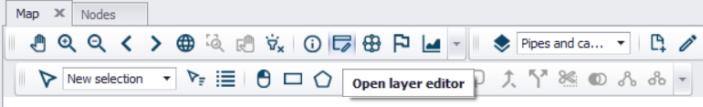
One way of automatically opening a table to the correct location (ID) is done through the Map view. Click on the tool, click on a location on the map (e.g. the pipe of interest) and the appropriate table will open in a new tab at the correct location showing the corresponding attributes.

Editing the Data in the Editor Table

Once the location to be edited is identified, there are a few ways to edit attributes.

Information can be manually typed into the form fields, where the input fields displayed correspond to where the small triangle appears on the row ID. Alternatively, values can be manually input into the table at the bottom of the screen.

The most useful method to edit data en masse is to use the Field calculator which is available by right clicking on a table header. An expression editor is then available where simple or complex expressions can be written to edit selected rows. If no rows are selected, the expression will be applied to the entire column.

 

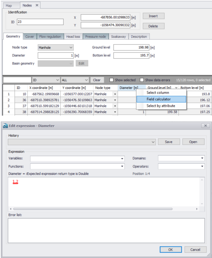
Figure: Editing data using the Field calculator

Another method of editing database values is to edit values within the Property and Result Explorer. Activate the Identify tool in the Map view, and click on the item of interest (e.g. node). In the table that appears as part of the identify tool, values can be directly edited and will be automatically synchronised with the map and database tables.

 

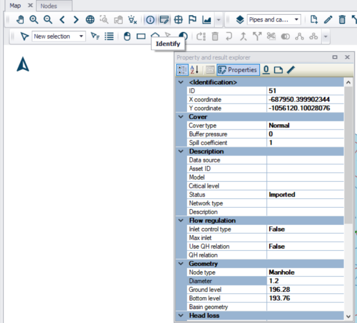
Figure: The database can be edited within the Identify tool

Note

Applying the Field Calculator with a PostgreSQL database from a distant server may be significantly slower than when working with a local database. This is an expected behaviour, and happens when the updated field triggers additional updates in other editors (e.g. when editing IDs, then all connected items must also get updated connection IDs), hence requiring additional communication time with the distant server.