2D Domain

The 2D Domain editor is where the computational grid or mesh for the 2D model is configured or defined.

 

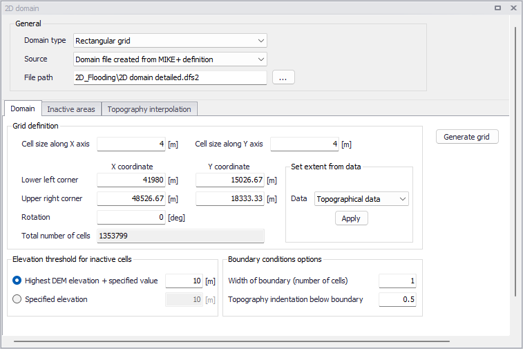
Figure: The 2D Domain editor

General

Define general properties for the 2D model computational grid under the General group box at the top of the editor.

Domain Type

Select the type of 2D computation grid to use in the project from the dropdown menu. In MIKE+, computational grids may be:

• Rectangular Grid: Made up of orthogonal, uniformly-spaced grid points representing the model domain. Related to MIKE *.dfs2 file types.
• Flexible Mesh: Made up of non-uniform triangular or quadrangular elements representing the model domain. Related to MIKE *.mesh file types.

 

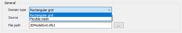
Figure: 2D domain type options

Source

The 2D computational grid may be may be directly specified in the editor with an existing file or may be configured and generated from MIKE+. The Source dropdown menu offers options for using a:

• Domain file created from MIKE+ definition: With this option, it is required to specify the extent of the 2D domain and its resolution, and finally interpolate topographical data onto the computational points.
• Existing domain file: With this option, an input 2D domain file must be supplied and will be used as is.

 

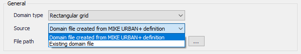
Figure: 2D domain source options

File Path

Depending on the Source and Domain Type specified, the File Path will refer to either the:

• Path and file name for the domain file to be generated from MIKE+: This is relevant for when the Source is ‘Domain file created from MIKE+ definition’.
• Path to the existing domain file: This is relevant for when Source is ‘Existing domain file’.

 

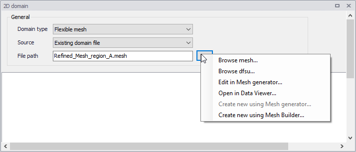
Figure: File path options

The ellipsis button (...) offers the following functions:

• Browse: Launches the file explorer for navigating to the desired location of the domain file to be created or the location of the existing domain file, when using the ‘Rectangular grid’ domain type.
• Browse mesh: Launches the file explorer for navigating to the desired location of the domain file to be created or the location of the existing domain file, when using the 'Flexible mesh' domain type.
• Browse dfsu: Launches the file explorer for navigating to the desired location of the existing domain file, when using the 'Flexible mesh' domain type and when the 2D domain should preferably be defined with element-centered topographical values. Only the first item from the selected *.DFSU file can be used.
• Edit grid in Grid Editor: Launches the Grid Editor to edit existing or previously-created rectangular grids.
• Edit in Mesh Generator: Launches the Mesh Generator to examine/edit existing or previously-created *.MESH files.
• Open in Data Viewer: Launches the Data Viewer to examine/edit existing or previously-created *.MESH files.
• Create new grid file: Launches the Grid Editor to create a new 2D rectangular *.DFS2 grid.
• Create new using Mesh Generator: Launches the Mesh Generator to create a new flexible mesh file.
• Create new using Mesh Builder: Launches the Mesh Builder to create a new flexible mesh file. You must be signed in to MIKE Cloud in order to access the Mesh Builder. Read Chapter 2.13 'Working with MIKE Cloud' in the MIKE+ Model Manager User Guide for more information.

Note

When the 2D Domain file is created from MIKE+ definition, and when this definition is changed in different alternative scenarios, it is highly recommended to save the 2D domain file with a different file name for each scenario. If this file name is instead kept unchanged, the resulting 2D domain file won't be updated right after switching scenario although the changes to its definition (e.g. in grid extent or inactive areas) will be changed for each scenario.

Domain

When creating new computational grids from MIKE+, the Domain tab is where basic properties for grid/mesh generation are defined.

Tab contents in the editor change depending on whether a Rectangular Grid or a Flexible Mesh shall be created.

Rectangular Grid

 

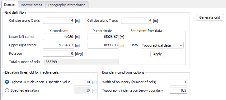
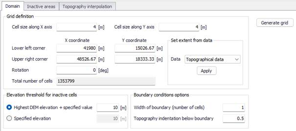
Figure: The Domain tab for configuring new rectangular grids

• Grid definition: Define the grid cell size along the x- and y-directions, and the extent of the 2D model domain. The extent may also be derived from available data layers, such as:
  • Topographical data: Based on the data layer(s) to be used in 2D topography interpolation. The data layers must be activated in the ‘Topography interpolation’ tab to be properly detected as ‘Topographical Data’.
  • Collection system network: The extent of the network of pipes and canals.
  • River network: The extent of the whole network of rivers
  • Active selection: The maximum extent of currently-selected model elements.
• Elevation threshold for inactive cells: Define the elevation value over areas that should remain inactive during 2D model computations. Inactive grid cells are excluded from computations.
  • Highest DEM elevation + specified value: The specified value is added to the maximum elevation value detected from the 2D domain file.
  • Specified elevation: Areas with terrain levels equal to or higher than the defined value are considered inactive.
• Boundary conditions options: Specify the width and grid cell levels at 2D boundary sections. 2D boundaries (i.e. closed and open boundaries) are located along edges of the 2D domain in MIKE+.
  • Width of boundary (number of cells): Define the width (in the direction transversal to the border of the domain) of 2D boundary edges in terms of number of grid cells. Grid size is defined under the ‘Grid definition’ section. This width is used for the indentation described below.
  • Topography indentation below boundary: The depth subtracted from the lowest cell level within the area with indented cells. The adjusted level in this lowest level is assigned to all other cells in the open 2D boundary area (figure below). This is used to apply a constant topography along the boundary and ensure that the boundary is e.g. always flooded.
  • Along the 2D model perimeter where no 2D boundary condition is applied, the ground elevation is automatically raised to the elevation threshold for inactive cells. This is to represent a closed boundary ensuring zero flow across the perimeter (also see the Raised areas in the figure below).
  • Along stretches where an open water level or discharge boundary is defined, the ground is lowered to a uniform level to ensure valid numerical computations at the boundary as open boundaries must be wet all the time (figure below).

 

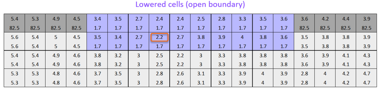
Figure: Example of automatic terrain level lowering along an open 2D boundary spanning 10 2D cells. In each 2D cell the original levels (upper values) and adjusted levels (lower values) are shown. The value of 1.7 m is taken from the lowest-level unadjusted cell in the area (i.e. 2.2 m encircled) minus the specified indentation (here 0.5 m).

Flexible Mesh

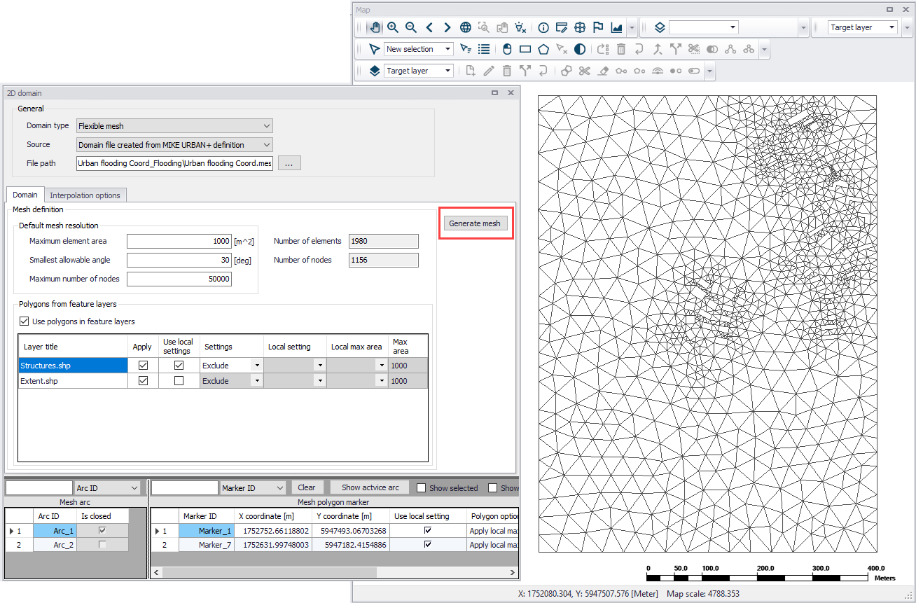
For flexible meshes, the Domain tab is where mesh resolution, overall extent, and local mesh area properties may be defined.

 

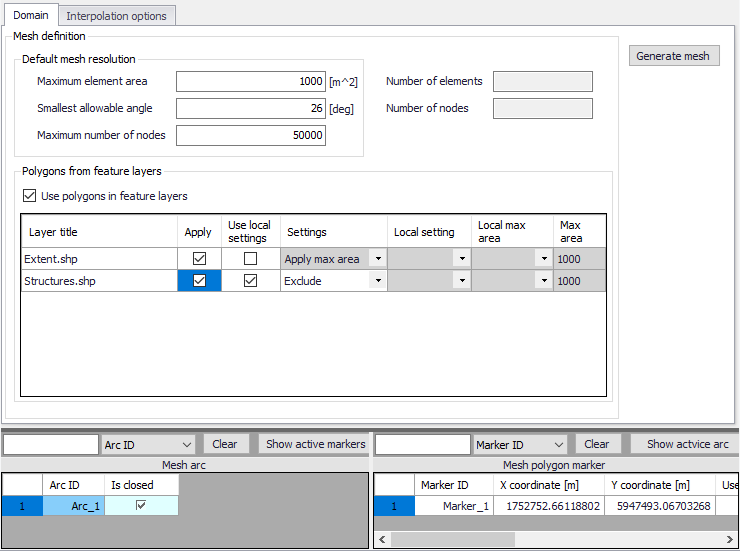
Figure: The Domain tab for configuring new flexible meshes

The first step to build a flexible mesh is to specify the ‘Default mesh resolution’, which will apply in locations where no local mesh resolution is defined. Under this ‘Default mesh resolution’ section, set values for various default mesh generation criteria. These include:

• Maximum element area: Area upper bound for elements in the mesh to be generated.
• Smallest allowable angle: Target smallest interior angle for elements in the generated mesh.
• Maximum number of nodes: Upper limit for number of element vertices in the mesh to be generated.

The second step is to define Mesh polygons and arcs, to apply local mesh resolutions. Polygons are used to define the overall extent of the mesh, as well as areas where local mesh settings shall be applied. These areas may be defined using:

• Feature layers: When the option 'Use polygons in feature layers' is active, polygons from feature layers may be used for the mesh generation. The layers must be added to the Map before use in mesh generation. Usable feature layers are automatically listed. Activate the 'Apply' option for layers to use and adjust the settings below:
  • Use local settings: If this option is not selected, the default mesh resolution will apply within the polygon: the effect of the polygons is limited to the fact that mesh elements will be somehow aligned to the polygons. If this option is selected, then local settings controlled by the following parameters will be applied in the polygons.
  • Settings. Three settings definitions are available:
  • Apply max area: For this setting, all polygons in the feature layer will use the same local mesh resolution, controlled by the value specified for the 'Max area'.
  • Exclude: For this setting, all polygons in the feature layer will be excluded from the mesh. Not other input is required.
  • Layer attributes: For this setting, each polygon in the feature layer may have its own local mesh resolution, which is controlled by the attributes of the layer. In the 'Local setting' column, it is required to select an attribute from the feature layer, containing the type of setting for each polygon: this must be a text attribute, and for each polygon the text must be either 'local area' or 'exclude' (case insensitive). In the 'Local max area' column, it is required to select an attribute containing the maximum element area for each polygon, to be used for polygons included in the mesh.

 

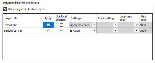
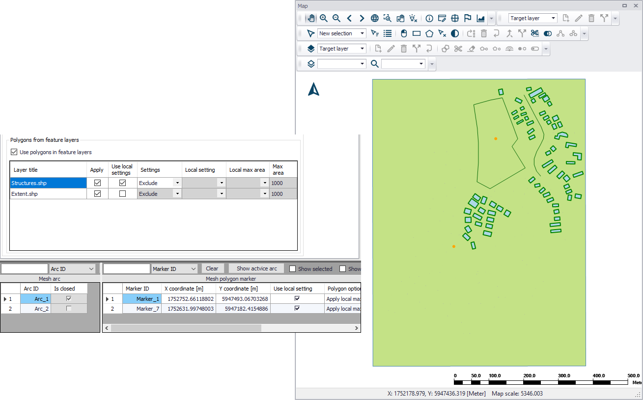
Figure: List of polygon features that may be used for mesh generation in the Domain tab

• Mesh arcs and polygon markers: Mesh arcs and polygon markers are drawn on the Map. Arcs are lines or polylines that are open or closed. Closed arcs have the same first and last nodes, to create a polygon. A polygon marker may be added within a polygon, in order to specify the local properties of the mesh in the polygon. A polygon without marker will be meshed with the default mesh resolution.

Define arcs and polygons on the Map using the Flooding Layer Editing toolbar or the Edit Features toolbox on the 2D Overland menu ribbon. Select ‘Mesh arc’ as the target layer from the toolbar and use the ‘Create’ tool to draw arcs on the map.

Mesh polygon markers define local mesh properties in the encapsulating polygon. A polygon may only have one polygon marker.

Records for defined domain definition layers (i.e. arcs and polygon markers) are shown in the table at the bottom of the 2D Domain editor. The 'Show active marker' button, in the table of arcs, may be used to find the marker located in a given closed arc: select the relevant arc in the table, press the button, and the number of the corresponding marker in the table will be highlighted in dark blue. Similarly, the 'Show active arc' button, in the table of markers, may be used to find the encapsulating arcs: select the relevant marker in the table, press the button, and the numbers of the corresponding arcs in the table will be highlighted.

 

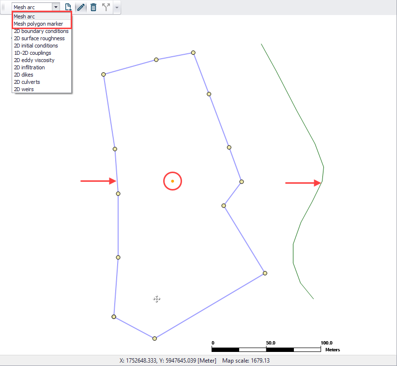
Figure: Define arcs and polygons on the Map via the Flooding Layer Editing toolbar. The figure shows a closed and open arc indicated by the arrows, and a polygon marker (encircled).

 

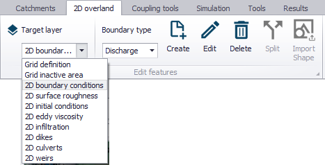
Figure: The Edit Features toolbox on the 2D Overland menu ribbon

 

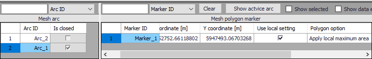
Figure: Mesh arcs and polygon markers grid table at the bottom of the 2D Domain editor

It may sometimes happen that a polygon from feature layers and a polygon defined by closed mesh arcs overlap (one being eventually fully included in the other one). In this case, the following rules apply:

• If one polygon is requested to be meshed and the other polygon is requested to be excluded from the mesh: then the priority is given to the polygon excluded from the mesh, and all the area covered by this polygon is excluded (even the parts covered by the other polygon).
• If the two polygons are requested to be meshed: priority is given to the polygon from the feature layer. In this polygon, the mesh will get the resolution requested for this polygon, even in the parts covered by the polygon defined with mesh arcs.
• If the two polygons are requested to be excluded from the mesh: the total area from the two polygons is excluded from the mesh.

Note

Building areas can be excluded from the simulation, in order to take the effect of the obstacles on the flow. However, if rainfall is to be applied on the 2D domain, the volume of rain falling on the buildings will not be accounted for. The use of 2D Infrastructures is an alternative solution to describe buildings, which can keep taking into account the rainfall volume falling on buildings.

Inactive Areas

This tab is accessible only when generating Rectangular Grids. It is where areas for inactive cells in the computational grid (other than closed boundaries) are defined.

Inactive cell values, as configured in the Domain tab (i.e. Elevation threshold for inactive cells), are assigned to these cells. These areas may be defined with:

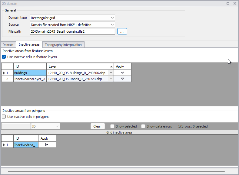
• Feature Layers: Polygon feature layers loaded to the Map prior to grid creation. The layers must be added to the Map before use. Then, use the 'Insert' button to start using a new feature layer as inactive area, and select the source layer from the drop-down list. Activate the ‘Apply’ option for layers to use and tick on the ‘Use inactive cells in feature layers’ option to use the applied layers during grid interpolation. Unticking the 'Apply' option allows to ignore a layer without removing it, e.g. for later reuse or for use in alternative scenarios only. All cells within a polygon from the applied layers will be excluded from the computation.

 

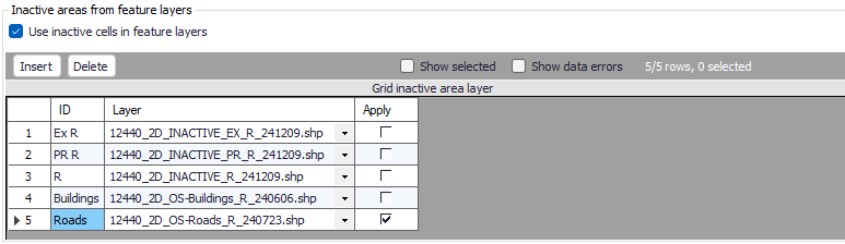
Figure: List of polygon features that may be used to define inactive cells for rectangular grids

• Polygons: Define inactive polygons on the Map using the Flooding Layer Editing toolbar or the Edit Features toolbox on the 2D Overland menu ribbon. Select ‘Grid inactive area’ as the target layer from the toolbar and use the ‘Create’ tool to draw polygon features on the map. Records for defined polygons are shown in the ‘Grid inactive area’ secondary table at the bottom of the Inactive Areas tab page.

 

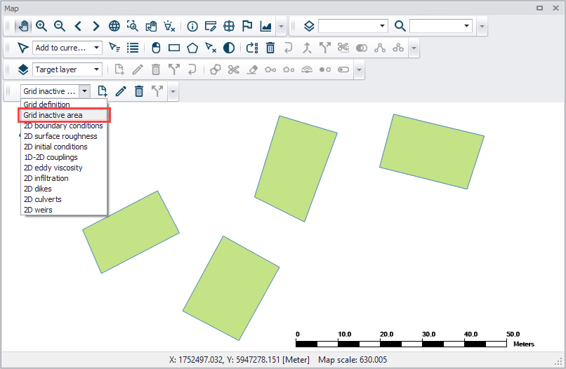
Figure: Use the Flooding Layer Editing toolbar to create Grid Inactive Area polygons on the map

 

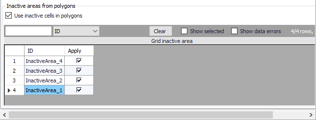
Figure: Grid inactive area secondary table at the bottom of the Inactive Areas tab page

Inactive area polygons for rectangular grids may be re-used as mesh area polygons for excluded areas during flexible mesh generation. A warning message is issued when switching from rectangular grid to flexible mesh domains after grid inactive areas have been created. Clicking on the ‘Yes’ button will add the previously-applied grid inactive areas to the mesh domain polygons.

 

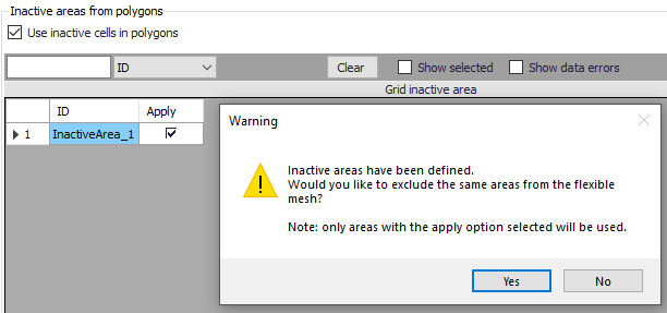
Figure: Warning message offering to option to use grid inactive areas a mesh domain polygons

Note

Building areas can be excluded from the simulation, in order to take the effect of the obstacles on the flow. However, if rainfall is to be applied on the 2D domain, the volume of rain falling on the buildings will not be accounted for. The use of 2D Infrastructures is an alternative solution to describe buildings, which can keep taking into account the rainfall volume falling on buildings.

Topography interpolation

The ‘Topography interpolation’ tab is where topographical data and methods for interpolating topographical values onto the generated computational grid or mesh are configured.

Perform interpolation only after the grid or mesh has been generated.

 

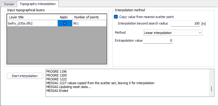
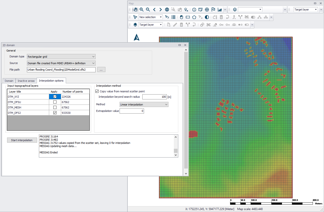
Figure: The Topography interpolation tab

Input Topographical Layers

Input topographical layers are sources of scatter data for interpolation of values onto the grid or mesh. The following file types may be used as input topographical layers in MIKE+:

• Raster Layers *.tif and *.tiff
• Raster Layer *.dfs2
• Feature Layer *.xyz
• Mesh Layers *.mesh and *.dfsu

Load these data layers into MIKE+ via the ‘Add layer’ function in the ‘Layers and Symbols’ View. These layers are added to the Map, and valid layers are added to the ‘Input topographical layers’ table in the 2D Domain editor.

Click on the ‘Apply’ column if the layer shall be used as a source of scatter data in the interpolation. The ‘Number of points’ column displays the number of scatter data points in the layer. This indicates the number of nodes for a *.MESH file, and the number of cells or elements for *TIFF, *.DFS2 or *.DFSU files, respectively.

 

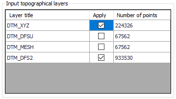
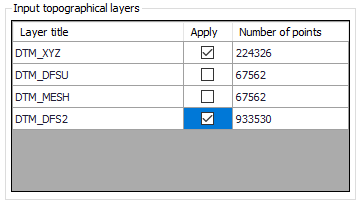
Figure: The Input Topographical Layers table on the Topography interpolation tab

For .dfs2, .dfsu and .mesh files, units of elevation data are controlled and specified in these files. For TIFF files, the unit must also be defined in the TIFF properties, and if the unit is not a valid unit or is undefined, elevation data will be assumed to be in meters. For .xyz files, the unit is selected while adding the file on the map.

Interpolation Method

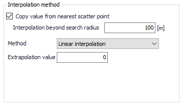
This section offers available options for interpolating values onto the grid or mesh. These include:

• Copy value from nearest scatter point: In this option, mesh node values are simply taken from the nearest scatter point (i.e. from active input topographical layers). This option can dramatically decrease interpolation time when a very dense set of scatter data points is available. This is because values are simply set from the nearest scatter points, and true interpolation is only performed for areas where scatter points are beyond the search radius. Mesh node points assigned a value in this way will not be included in the overall interpolation. The search radius from a mesh node to the nearest scatter point is set via the ‘Interpolation beyond search radius’ parameter. Set a reasonable search distance based on scatter data resolution.
• Method. The available interpolation methods are:
  • Linear Interpolation: For each mesh node to be interpolated, a surrounding triangle based on scatter points is determined, and a linear interpolation based on the scatter point values is made.
  • Natural neighbour interpolation: Is a geometric estimation technique that uses natural neighbourhood regions generated around each node. The natural neighbourhood regions are determined by creating a triangulated irregular network from the scatter data points. It is particularly effective in dealing with a variety of spatial data themes exhibiting clustered or highly linear distributions. Natural neighbour method extrapolation beyond the extent of the scatter data may be enabled and controlled through the ‘Extrapolate to ...% beyond envelope of scatter data’ parameter. The points will be placed at the lower left, upper left, lower right and upper right corner of the workspace area, respectively. The parameter specifies the distance from the four points to the data extent area. The water depth value at the four points will be defined as the extrapolation value.

 

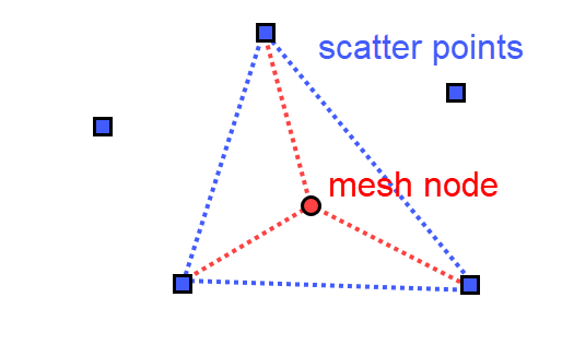
Figure: Illustration of the linear interpolation method for deriving topography values for mesh nodes from input scatter points

 

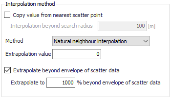
Figure: Natural neighbour interpolation parameters

 

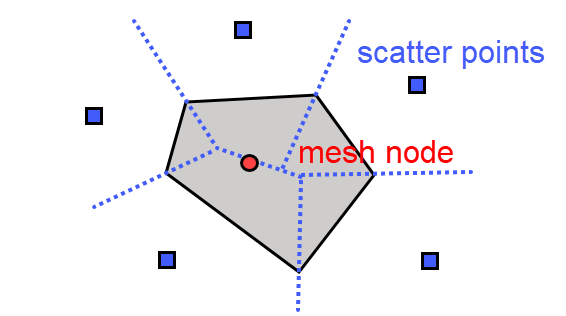
Figure: Illustration of the natural neighbour interpolation method for deriving topography values for mesh nodes from input scatter points

• Extrapolation value: Specify a value to be used when the program needs to extrapolate values beyond configured interpolation settings in the model.

Start Interpolation

Click on the ‘Start Interpolation’ button to launch the interpolation process. The status of the interpolation process is indicated in the progress window.

 

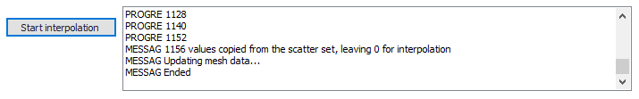
Figure: The Start Interpolation button and progress log window

Creating a Rectangular Grid Workflow Example

1. Load desired input topographical layers for 2D grid interpolation into the MIKE+ project.

2. On the 2D Domain editor, choose a ‘Rectangular grid’ domain type and ‘Domain file created from MIKE+ definition’ as source. Specify the file name and path for the domain file to be created.

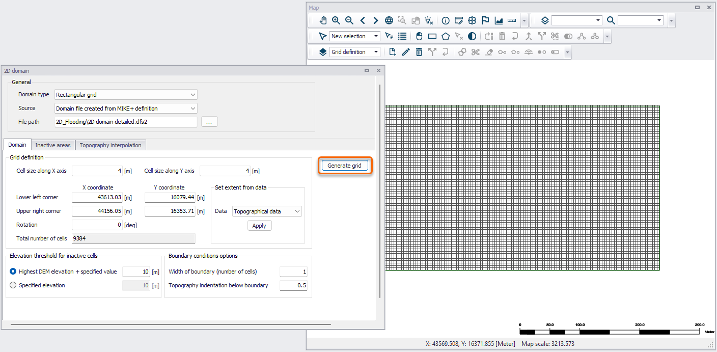
3. Configure grid domain parameters. Specify grid cell size along the x and y directions, and define the domain grid extent. You may choose to set the extent from Topographical data. If so, ensure that the appropriate topographical data layer is activated in the ‘Topography interpolation’ tab. You may also chose to define the grid extent by drawing it on the map. In the 2D overland ribbon, select the 'Grid definition' layer to draw a rectangle defining this extent. While editing this rectangle on the map, it is possible to resize and rotate it.

4. Customize other parameter values on the Domain tab, such as those under the ‘Elevation threshold for inactive cells’ and ‘Boundary condition options’ sections, if so desired. More details on these options are described in chapter Domain.

 

1. Click on the ‘Generate grid’ button on the Domain tab page.

 

1. Examine the generated grid. Adjust grid sizes and extent, as needed. Re-generate the grid after changes to grid parameters.

2. Define inactive areas, if any. If inactive areas shall be defined for the 2D domain, specify them as polygons on the Map, or load polygon feature layers that represent them into the project (see chapter Inactive areas for more details). Make sure to activate the appropriate tick boxes to apply the desired feature layers as inactive areas in the subsequent interpolation.

 

1. Configure interpolation parameters. Access the ‘Topography interpolation’ tab page. Select the input topographical layers to use in the interpolation.

 

1. Choose the preferred interpolation method. More details on the methods are described in chapter Topography interpolation.

 

1. Click on the ‘Start interpolation’ button. A progress bar appears, and the status of the process is shown on the log window.

Creating a Flexible Mesh Workflow Example

1. Load desired input topographical layers to be used for 2D mesh value interpolation into the MIKE+ project.

2. On the 2D Domain editor, choose a ‘Flexible mesh’ domain type and ‘Domain file created from MIKE+ definition’ as source. Specify the file name and path for the domain *.mesh file to be created.

3. Configure mesh domain parameters. Define the mesh extent, and any local mesh areas via loaded polygon feature layers, or mesh arcs and polygons drawn directly on the Map. Pre-loaded feature layers are listed under the ‘Polygons from feature layers’ secondary table in the middle of the page, while arcs and polygons drawn on the Map are listed on the table at the bottom of the editor. More details on defining mesh areas are found in chapter Flexible Mesh.

 

1. Customize other meshing parameters on the Domain tab, such as ‘Maximum element area’ and ‘Smallest allowable angle’, if so desired. More details on these options are described in chapter Flexible Mesh).

2. Create a mesh by clicking on the ‘Generate mesh’ button on the Domain tab page or in the 2D overland tab in the ribbon.

 

1. Examine the generated computational mesh. Adjust element sizes, the extent, or mesh areas using arcs and polygons, as needed. Re-generate the mesh after changes to meshing boundaries and parameters.

2. Configure interpolation parameters. When ready to finalize the 2D mesh, access the ‘Topography interpolation’ tab page to begin interpolating topographical values onto the mesh. Select the input topographical layers to use in the interpolation.

 

1. Choose the preferred interpolation method. More details on the methods are described in chapter Topography interpolation.

 

1. Click on the ‘Start interpolation’ button. A progress bar appears, and the status of the process is shown on the log window.