PID Parameters
The PID Parameters Editor
This editor is used to define the functions for PID (Proportional Integral Differential) control. PID controls can apply to various controllable parameters, either from collection system structures or from river structures, e.g. weir crest level, pump flow, etc. Independently of the choice of the controlled variable, the PID algorithm adjusts the settings of the regulator according to the current error between the specified setpoint and the actual value of the controlled variable.
A single PID set can be used in multiple actions.
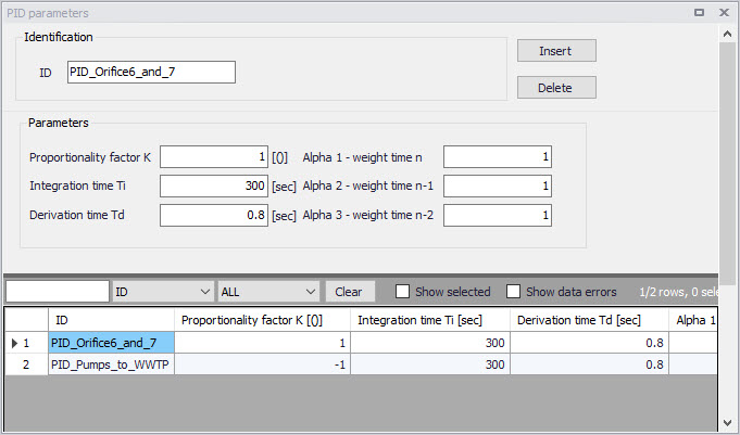
Figure: The PID Parameters editor
ID
Each set of PID settings is identified with a unique ID. This is how the PID parameter set is accessed from other dialogs.
Proportionality Factor, Integration Time, and Derivation Time
The 3 main parameters for the PID control. These parameters are further discussed in the section below Calibration of the PID Constants.
Alpha-1, Alpha-2 and Alpha-3
Weighting factors for time level n, n-1 and n-2. These parameters are further discussed in the section below Calibration of the PID Constants.
Calibration of the PID Constants
Tuning of the PID constants (Ti, Td and K) is not a straightforward task. Understanding the theoretical background and the numerical solution of the control equation would be beneficial in this process.
The following values may be used as a guide, suggesting typical values of the PID constants and weighting factors.
| Parameters | Pumps | Gates | Weirs |
|---|---|---|---|
| Ti | 300 sec. | ||
| Td | 0.8 sec. | ||
| K (Setpoint downstream of device) | 1 | 1 | -1 |
| K (Setpoint upstream of device) | -1 | -1 | 1 |
| Alpha-1 | 1 | 1 | 1 |
| Alpha-2 | 1 | 0.7 | 0.7 |
| Alpha-3 | 1 | 1 | 1 |
Table: Summary of typical values for PID constants and weighing factors
Note
The sign on the K-factor is very important. If it is wrong it will cause the control function not to work at all since the device will typically move to one of the extreme positions and stay there until the end of the simulation.
The three figures below show examples of how the actual variable (flow or water level) can fluctuate around the setpoint as a consequence of PID constants values. Each figure has three different graphs depending on whether the constant is too high, too low, or adequate.
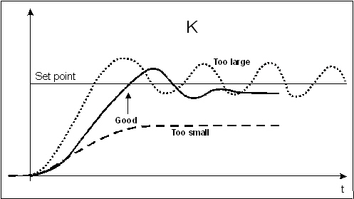
Figure: Fluctuations around the setpoint depending on the size of the proportionality factor, K
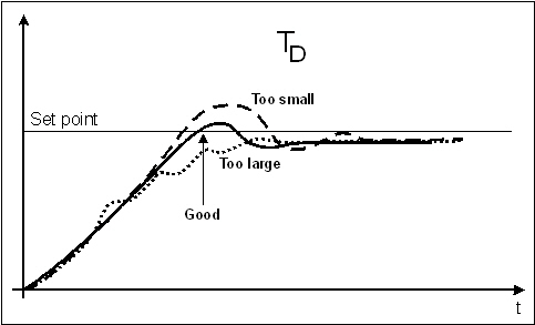
Figure: Fluctuations around the setpoint depending on the size of the derivation time, Td
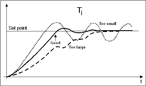
Figure: Fluctuations around the setpoint depending on the size of the integration time, Ti