Cross sections

The 'Cross sections' editor defining conduits' cross-sections, when this cross section changes along the conduit. This is used to describe natural channels with multiple cross sections along a single "pipe", when this pipe is defined with the type 'Natural channel' in the 'Pipes and canals' editor.

These cross sections data are stored in an external cross section file with the file extension .xns11.

Cross section tree

The cross section tree window in the tabular view shows the list of all cross sections in the setup. The data are stored in an external cross section file with the extension .xns11.

In the tabular view it is possible to see all the cross section in the setup. In the first column, cross sections are identified by their branch name, topo ID and chainage.

Clicking a cross section in the tree view will show the details of this cross section on the right-hand side of the Tabular view.

Right-clicking in the first column gives access to options to edit the cross sections. The options offered in the contextual menu depend on where you clicked in the tree view. For instance clicking on a single chainage allows editing the corresponding cross section only, whereas clicking on the topo ID or on the branch name allows editing all or a selection of cross sections.

The “Move...” feature allows to move cross sections to different locations, by changing either the branch name, topo ID and/or chainage. When selecting the “Move...” feature, a dialogue will be displayed. Where the “From” groupbox indicates with cross sections are being moved and where the “To” groupbox indicates the final destination which has been specified by the user.

 

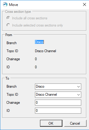
Figure: Dialogue for moving a cross section

The “From” groupbox shows the original chainage only when moving a single cross section. It shows the topo ID only when moving a single cross section or a group of sections from a given topo ID.

The upper part of the dialogue is only active when selecting ‘Move…’ from a branch name or a topo ID. It allows selecting between moving all the cross sections of the branch / topo ID, or only the selection. These options are therefore not relevant for moving a single cross section.

The ‘Copy…’ feature is similar to the ‘Move…’ one except that the original cross sections are kept at their original location.

To insert a cross section, it is possible to use the ‘Insert blank cross section’ feature, which allows creating a cross section on any branch and for any topo ID, which therefore have to be specified as shown in the figure below.

 

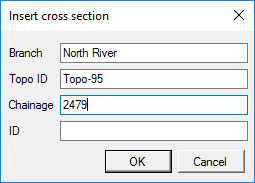
Figure: Insert a blank Cross Section

Alternatively, right-clicking on the branch name or topo ID allows inserting a cross section respectively in the corresponding branch or the corresponding topo ID. In that case the branch name and eventually the topo ID are automatically filled, as illustrated in the figure below.

 

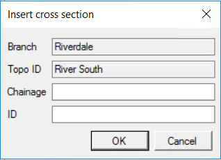
Figure: Dialogue for inserting a cross section in a selected topo ID

It is possible to insert an interpolated cross section, by right-clicking and selecting 'Insert interpolated cross sections'. This opens up the dialogue illustrated in the figure below, where the branch name and Topo ID where the interpolation is to be conducted must be selected. It is possible to interpolate a single cross section at a given chainage or multiple cross sections. In the latter case a maximum distance between the interpolated cross sections must be specified, along with the range of chainages.

Similarly there are multiple options for deleting cross sections. Right-clicking on a single cross section gives access to the ‘Delete this cross section’ feature. Clicking on the topo ID allows deleting either all cross sections under this topo ID (using the feature ‘Delete topo ID’) or only the selected sections under this topo ID (using the feature ‘Delete selected in this topo ID’). Finally, clicking on the branch name allows deleting either all cross sections under this branch (using the feature ‘Delete river’) or only the selected sections under this branch name (using the feature ‘Delete selected in this river’).

 

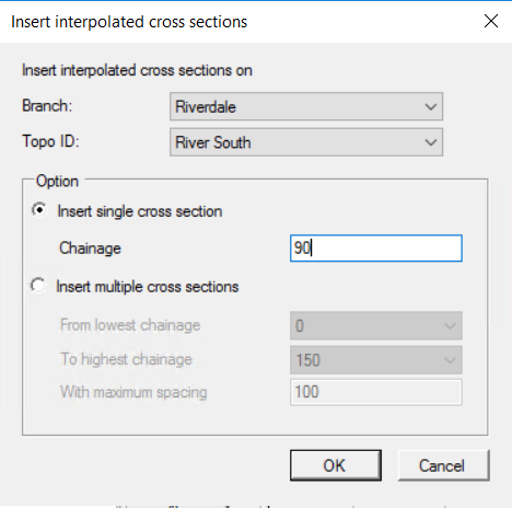
Figure: Dialogue for inserting an interpolated cross section

Similarly there are multiple options for deleting cross sections. Right-clicking on a single cross section gives access to the ‘Delete this cross section’ feature. Clicking on the topo ID allows deleting either all cross sections under this topo ID (using the feature ‘Delete topo ID’) or only the selected sections under this topo ID (using the feature ‘Delete selected in this topo ID’).

Cross section properties

General

The General tab contains options and data which relevant for all or part of all the cross sections.

Recompute all. The ‘Recompute all’ button recomputes processed data for all the cross sections.

Recompute selected. The ‘Recompute selected’ button recomputes processed data for the selected cross sections (those having the ‘Select’ checkbox checked) only.

Cross-section filename. Cross sections are stored in a cross section file, with the xns11 file extension. Click the ‘…’ button to either select an existing file, create a new one or refresh the content of the file.

Draw history on plots. When this option is checked, watermarks are added as a history of previous cross sections drawn on the ‘Cross section plot’ and the ‘Processed data plot’. This feature allows comparison of multiple cross sections on a single scale.

Coordinates

The ‘Coordinates’ tab provides the list of vertices defining the location of the cross section (i.e. the polyline shown on the map). Each row describes a point identified with its X and Y coordinates expressed in the coordinate sys tem used for features in the setup. The ‘S’ column provides the horizontal distance of each vertex along the polyline from its left end. These vertices don’t have to match the list of points provided in the ‘Raw data’ tab.

When cross sections have been created from the Map view, the table is automatically filled with all vertices defining the location of the polyline and one point at the intersection with the branch.

Apply. When coordinates are provided in the table, the ‘Apply’ option can be checked. When it’s checked, cross sections are displayed on the map based on the defined coordinates otherwise the cross section is displayed perpendicular to the branch at the specified chainage.

Raw data

The ‘raw data’ tab provides the list of points defining the topography of the river bed along the cross section. These points don’t have to match the list of vertices provided in the ‘Coordinates’ tab.

The ‘S’ column provides the horizontal distance of each point along the cross section, from the left end of the cross section. The ‘Z’ column provides the elevation of the points.

The ‘+’ button above the table can be used to insert a new line at the bottom of the table, while the ‘-‘ button can be used to delete the active line.

Markers. Markers may be assigned to points in the ‘Marker’ column of the table. Markers can be assigned in two different manners: the first one is to click an element in the ‘Marker’ column, which opens a marker dialogue as shown in the figure below from which a requested marker number can be assigned for the selected point.

 

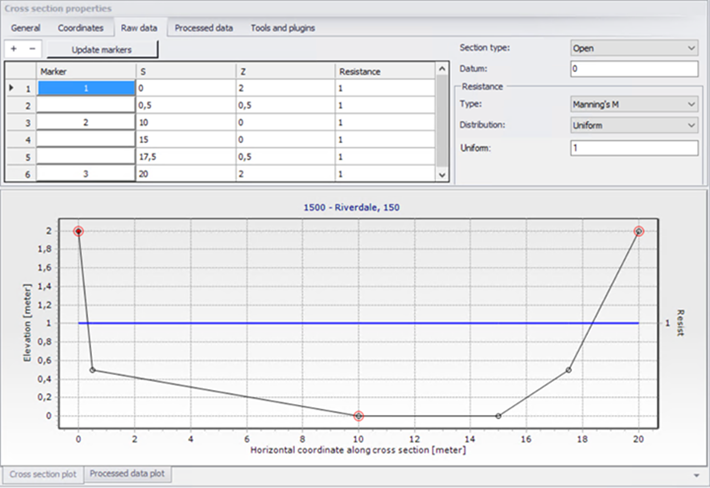
Figure: The marker options for the cross section type X-Z-R-M

 

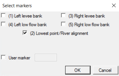
Figure: Selection of markers

A number of markers may be set in this dialogue:

Left and right levee mark (Markers 1 & 3): defines the extent or the active part of the cross section used for the calculations. Default placement of marker 1 and 3 is to apply marker 1 in the very first point in the raw data and marker 3 at the very last point of the raw data. Placing any of these markers at different locations will limit the extent of the active part of the cross section such that only the part of the cross section in between markers 1 and 3 is included in the simulation (that is, Processed data are only calculated for cross section data in between these markers).

Left and right low flow bank (Markers 4 & 5): defines the extent of the low flow channel. The markers influence the calculation of the processed data. If defined, the section is internally divided into three major ‘slices’ at markers 4 and 5 positions and the resulting processed data for such a section is a sum of integration results of three sub-parts of the section instead of calculating a result from one single, large section. Additionally, markers 4 and 5 can be used to define the extent of the low flow channel which is used with the ‘High/low flow zones’ description of the resistance distribution in the raw cross section data.

Lowest point/River alignment (Marker 2): marker 2 typically define the lowest point of the river section, or the location of the intersection with the branch. Marker 2 settings does not affect the calculations at all. Instead, it serves primarily the Map view for placement of cross sections which have no coordinates defined. It is therefore recommended to define the correct position of marker 2 in all sections.

User marker: any number above 7 may be used as a user marker. User markers do not impact the simulation results. They are an option for indicating a specific point in a cross section e.g. the location of a measurement gauge.

Marker locations must be defined such that marker 1 is defined to the left of marker 3 in the raw data table.

Update markers: This button updates markers 1, 2 and 3 in the current cross section, which are respectively placed at the left end point, lowest point and right end point.

Section Type. The type of cross section is set here. Four options are available:

• Open section: the typical setting for river cross sections.
• Closed irregular: closed sections with arbitrary shape.
• Closed circular: closed circular section shape where the geometry is only defined by the diameter.
• Closed rectangular: closed rectangular section shape where the geometry is only defined by the width and height.

Datum. A datum value may be entered here. The datum is normally used for adjusting the levels of the cross sections such that they conform to a specific reference datum in the model area. The datum value is added to all elevations in the ‘Raw data’ tab. The datum is also used for circular and rectangular sections, to set the elevation of the bottom level of the cross section.

Resistance – Type. Multiple options exist for defining the desired type of resistance method in the cross sections. The following types are available

Relative resistance: the resistance is given relative to the resistance number specified in the ‘Bed resistance’ menu. The resistance value specified in the cross section for this resistance type is therefore a coefficient.

A coefficient higher than 1 will increase the actual roughness of the channel (river) bed, whereas a coefficient lower than 1 will decrease the actual roughness. So when the resistance type is Manning (M) in the 'Bed resistance' menu, then the Manning's M value is divided by this coefficient.

When the resistance type is Manning (n), then the Manning's n value is multiplied by this coefficient.

• Manning’s n: the resistance number is specified as Manning’s n in the unit s/m(1/3).
• Manning’s M: the resistance number is specified as Manning’s M in the unit m(1/3)/s (Manning’s M = 1/Manning’s n).
• Chezy number: the resistance number is specified as Chezy number in the unit m(1/2)/s.
• Darcy-Weisbach (k): the resistance is specified in the form of an equivalent grain diameter.

Resistance – Distribution. This distribution type defines the description of the transversal resistance across the cross section. Three options are available:

• Uniform: a single resistance number will be applied uniformly throughout the cross section.
• High/Low flow zones: three resistance numbers are to be specified. The ‘Left high flow’ number applies between markers 1 and 4, the ‘Right high flow’ number applies between markers 5 and 3, and the ‘Low flow’ number between markers 4 and 5. If marker 4 and 5 do not exist the low flow resistance number will apply uniformly throughout the cross section.
• Distributed: the resistance number is to be specified for each point, in the raw data table in the ‘Resistance’ column. The value specified for a given point applies uniformly between this point and the previous one.

Processed data. The ‘Processed data’ tab displays the hydraulic characteristics of the cross section which are used during the simulation. These processed data provide the values of cross section area, radius, width, bed resistance and conveyance as a function of the water level. The details of these variables are provided below:

• Level: levels for which processed data are calculated in the cross section.Default levels definition range from the lowest z-value and up to the highest z-value in the raw data table.
• Cross section area: effective cross sectional flow area calculated from the raw data. Effective area is determined from the total flow area adjusted by eventual relative resistance values different from 1 in the raw data tab (see MIKE 1D Reference manual).
• Radius: a resistance or hydraulic radius depending on the selected type in the ‘Radius type’ drop-down list.
• Storage width: width of the water surface for the given water level.
• Resistance: this factor can be used to apply a level dependent, variable resistance in the cross section. The resistance factor can contain the following two types of values depending on the Resistance Type definition in the raw data tab:
  • Resistance type defined as relative resistance factor: in this case, the resistance value is interpreted as a factor by which the resistance numbers defined in the 'Bed resistance' menu will be multiplied or divided during the calculation, in order to establish a level dependent resistance in the section. That is, the resistance factor works as a level dependent resistance scaling factor in the current section. It is important to notice in the case of relative resistance type, that a factor higher than 1 will increase the actual roughness of the river bed, whereas a factor lower than 1 will decrease the actual roughness. So when the resistance type is Manning (M), then the Manning's M value is divided by this factor. When the resistance type is Manning (n), then the Manning's n value is multiplied by this factor.
  • Resistance type defined as absolute resistance number (Manning’s n, Manning’s M or Chezy number): in this case, the resistance column contains the actual resistance number applied in the simulation. The resistance column can therefore have values of either Manning’s M, Manning’s n or Chezy numbers in this case.
• Conveyance: the conveyance values are not used in the simulation but is primarily displayed as part of the processed data for the purposes of checking that the conveyance is monotonously increasing with increasing water level, which is one of the key assumptions for the open water hydraulics.

Additionally, an additional storage area may also be defined manually, again as a function of the water level. The purpose of the additional storage area is to include an additional volume of storage in the cross section, which is not represented by the geometry in the raw data. The calculated water level in this additional storage remains strictly the same as in the cross section. This is useful for representing small storage’s associated with the main branch such as a lakes, bays and small inlets. The additional storage area values describe the area of the water surface for a given water level. Additional storage areas are always user-defined: they will never be given a value from the automatic processing of the raw data. During the simulation, the processed data will be interpolated in order to cover the full range of water levels encountered during the simulation.

Note

Processed data are essentials in the simulation, as they describe the hydraulic aspects of the cross sections. Hence, it is important to inspect processed data and make sure that accurately describe these hydraulic parameters.

It is for example important to make sure that their plots are smooth in order to correctly reproduce the progressive changes with changing water levels. If the plots show abrupt changes, it may be necessary to edit the levels at which processed data are computed. Additionally, a situation where the conveyance column is not monotonically increasing with water levels can relatively easily occur, especially in the case of some closed sections or in situations where the section geometry includes a sudden width increase and the radius type has been selected to ‘Hydraulic radius’. Should this situation occur, then it is strongly recommended (not to say a strict requirement) that time is spent on adjusting the section characteristics such that a monotonically increasing conveyance curve is obtained. If not, there is a very significant risk of obtaining instabilities in the simulation for water levels in the range where the non-increasing conveyance values are present.

Typical options for optimising the cross section characteristics in the situation of an open section is to use the ‘Resistance radius’ type instead. Alternatively, an option using the ‘Hydraulic radius’ type is to manually subdivide the section into several ‘slices’ by adjusting the relative resistance numbers in the raw data at locations where the section’s shape significantly changes (e.g. changing a relative resistance value from 1.000 to 1.001 ‘forces’ the processed data calculator to divide the integration of the processed data into several slices and the non-monotonically increasing conveyance curve can normally be resolved from this.

It is important to notice that the conveyance numbers presented in the conveyance column are actually not the ‘True’ conveyance values. Depending on the choice of resistance type in the ‘Processed data’ tab, the ‘True’ conveyance may depend on the resistance values specified in the ‘Bed resistance’ menu. However it has been decided to present conveyance values which does not include these resistance number. Consequently, the conveyance shown in the processed data does not reflect the true conveyance, but is primarily offered as a possibility for analysing the ‘conveyance trend’ as a function of water levels in the cross sections. And these should be monotonically increasing with water levels to secure a healthy output from the simulations.

The ‘+’ button above the table can be used to insert a new line in the table, while the ‘-‘ button can be used to delete the active line.

Allow for recalculation. When this option is checked, the table may be automatically recomputed. Data are recomputed when changes are applied to the cross section’s properties, when the ‘Recompute’ button in the current window is pressed. In case the processed data have been manually adjusted, it may be necessary to uncheck this option in order to make sure to keep them unchanged afterwards.

Processed data are also recomputed when the setup is saved when ‘Allow for recalculation’ is checked.

Recompute. This button is only active when the option ‘Allow for recalculation’ is checked. Pressing this button recomputes all the processed data in the table.

Radius type. The radius type may be chosen between the three following options:

• Resistance radius: a resistance radius formulation is used.
• Effective area, hydraulic radius: a hydraulic radius formulation where the area is adjusted to the effective area according to the relative resistance variation.
• Total area, hydraulic radius: a hydraulic radius formulation where the total area is equal to the physical cross sectional area.

Number of levels. The desired number of processed data levels. The automatic level selection method may not use the full number of level specified. This will occur when a smaller number of levels is sufficient to describe the variation of cross sectional parameters.

Angle correction. An angle correction may optionally be applied to the cross section. The correction may be used for situations where the cross section profile isn’t perpendicular to the center line of the river. To activate the correction, the ‘Apply’ checkbox must be checked, and the angle must be manually specified.

The correction applied is simply a projection of the cross sectional profile on the normal to the thalweg of the river i.e. the correction reads

 

Where is illustrated below

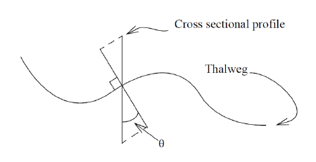
Figure: Definition sketch of the correction angle

Note

The correction of X-coordinates is not reflected in a change of S values in the raw data table, but only in the processed data table.

Cross section plot

The graphical view presents either a single plot for the current cross section, or eventually a number of plots from different sections if the ‘Draw history on plots’ option in the ‘General’ tab is active. The curve represents the values defined in the raw data table, with the X axis describing the S values and the Y axis describing Z values plus the datum value.

Points shown with red circles on the plot indicate the locations of markers 1, 2 and 3.

The blue curve describes the resistance value for the current cross section.

To control the settings and appearance of the plot, a number of facilities are available through a contextual menu. To open the pop-up menu point to the graphical view with the mouse cursor and press the right mouse button. A pop-up menu as presented in figure below will appear.

 

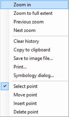
Figure: Contextual menu for the cross section plot

The pop-up menu includes the following three feature groups:

• The first group of features relates to the zooming facilities: from here the zoom in, zoom to full extent and the previous / next zoom facilities are available.
• The second group of features relates to the appearance and export of the graphical view. From here you can therefore export the image to the clipboard or to an image file on the disk, and you can also print it. Additionally the symbology dialogue allows changing the display settings of the plot.
• The third group of features relates to editing the active cross section's raw data on the plot. The following functions are available:
  • Select: when this mode is active, it is possible to select a cross section's point on the plot, which makes this point active in the raw data table.
  • Move points: when this mode is active, it is possible to move a point graphically from the plot. The raw data table will be updated accordingly.
  • Insert: when this mode is active, new cross section's point may be added. Inserted points are interpolated between two existing points, and may be moved afterwards.
  • Delete: when this mode is active, points may be deleted from the plot.

Processed data plot

The graphical view presents either the data for the current cross section only, or eventually for a number of cross sections if the ‘Draw history on plots’ option in the ‘General’ tab is active. The curve represents the values defined in the processed data table, with the Y axis describing the level values and the X axis describing one of the other items from this table (either area, radius, width, additional storage area, resistance or conveyance). The plotted item is controlled by the drop-down list above the plot.

To control the settings and appearance of the plot, a number of facilities are available through a contextual menu.