Demand Predictions

A list of the Demand predictions editor's attributes follows with a short description given for each one. Demand predictions allow you to use the demand prediction module that can predict future water consumptions (for an individual demand or for a zone) based on three methods:

• Statistical Winter-Holt method
• Machine learning
• 5-weeks method.

Insert

This button is used to insert a new row into the list.

Delete

This button is used to delete the selected row from the list.

 

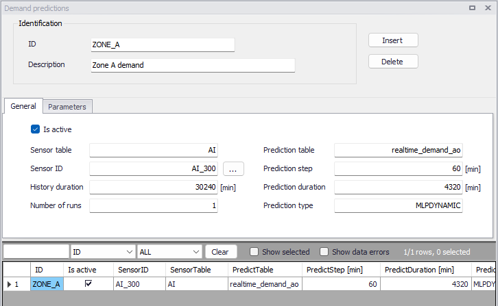
Figure: The Demand predictions editor for the Online analysis

The editor attributes are described below.

Is active

This check box allows the user to toggle the Active status of the demand prediction on and off.

Sensor table

Name of the sensor table (input to demand prediction).

Sensor ID

Name of the sensor with demand data to be used for prediction.

Prediction table

Name of the output table for predicted demands.

Prediction step

Time step used for demand prediction time series.

Prediction duration

Duration of the demand prediction time series.

History duration

Duration of past data used for demand prediction.

Prediction type (method)

Demand prediction type: HOLTWINTERS or MLPDYNAMIC or 5WEEKS.

Number of runs

• HOLTWINTERS: always 1
• MLPDYNAMIC: number of repeated runs to obtain the margins for uncertainty, the demand prediction will contain average values.
• 5WEEKS: always 1

PARAM1

• HOLTWINTERS: "trend". Type of trend component: "add", "mul", "additive", "multiplicative".
• MLPDYNAMIC: "activation". Activation function for the hidden layer: 'identity', 'logistic', 'tanh', 'relu':
  • 'identity', no-op activation, useful to implement linear bottleneck, returns f(x) = x
  • 'logistic', the logistic sigmoid function, returns f(x) = 1 / (1 + exp(-x)).
  • 'tanh', the hyperbolic tan function, returns f(x) = tanh(x).
  • 'relu', the rectified linear unit function, returns f(x) = max(0, x)
• 5WEEKS: alpha value for the exponential smoothing, e.g. 0.12. The exponential smoothing is defined as follows: Q(t) = alpha Q(t) + (1-alpha)Q(t-1).

PARAM2

• HOLTWINTERS: "seasonal". Type of seasonal component: "add", "mul", "additive", "multiplicative".
• MLPDYNAMIC: "hidden_layer_sizes". The ith element represents the number of neurons in the ith hidden layer: tuple, length = n_layers - 2. Default = 100.
• 5WEEKS: not used (leave empty).

PARAM3

• HOLTWINTERS: "seasonal_periods". The number of periods in a complete seasonal cycle, e.g., 4 for quarterly data or 7 for daily data with a weekly cycle.
• MLPDYNAMIC: "solver". The solver for weight optimization: 'lbfgs', 'sgd', 'adam'. Note: The default solver 'adam' works pretty well on relatively large datasets (with thousands of training samples or more) in terms of both training time and validation score. For small datasets, however, 'lbfgs' can converge faster and perform better.
  • 'lbfgs' is an optimizer in the family of quasi-Newton methods.
  • 'sgd' refers to stochastic gradient descent.
  • 'adam' refers to a stochastic gradient-based optimizer proposed by Kingma, Diederik, and Jimmy Ba
• 5WEEKS: not used (leave empty).

PARAM4

• HOLTWINTERS: not used, leave empty
• MLPDYNAMIC: "learning_rate". Learning rate schedule for weight updates: 'constant', 'invscaling', 'adaptive'.
  • 'constant' is a constant learning rate given by 'learning_rate_init'.
  • ‘invscaling' gradually decreases the learning rate learning_rate_ at each time step 't' using an inverse scaling exponent of 'power_t'. effective_learning_rate = learning_rate_init / pow(t, power_t)
  • 'adaptive' keeps the learning rate constant to 'learning_rate_init' as long as training loss keeps decreasing. Each time two consecutive epochs fail to decrease training loss by at least tol, or fail to increase validation score by at least tol if 'early_stopping' is on, the current learning rate is divided by 5.
• 5WEEKS: not used (leave empty).

PARAM5

• HOLTWINTERS: not used, leave empty
• MLPDYNAMIC: "learning_rate_init". The initial learning rate used. It controls the step-size in updating the weights. Only used when solver='sgd' or 'adam'. default=0.001.
• 5WEEKS: not used (leave empty).

PARAM6

• HOLTWINTERS: not used, leave empty
• MLPDYNAMIC: "max_iter". Maximum number of iterations. The solver iterates until convergence (determined by 'tol') or this number of iterations. For stochastic solvers ('sgd', 'adam'), note that this determines the number of epochs (how many times each data point will be used), not the number of gradient steps. Default=200.
• 5WEEKS: not used (leave empty).

PARAM7

• HOLTWINTERS: not used, leave empty
• MLPDYNAMIC: "n_iter_no_change". Maximum number of epochs to not meet tol improvement. Only effective when solver='sgd' or 'adam'. default=10.
• 5WEEKS: not used (leave empty).

PARAM8

• HOLTWINTERS: not used, leave empty
• MLPDYNAMIC: "tol". Tolerance for the optimization. When the loss or score is not improving by at least tol for n_iter_no_change consecutive iterations, unless learning_rate is set to 'adaptive', convergence is considered to be reached and training stops. default=1e-4.
• 5WEEKS: not used (leave empty).

SensorMult

This is the multiplier "k" that will be used to multiply the SCADA value before using it in the model update. Model value = scada value * k + n.

SensorOffset

This is the offset "n" that will be added to the SCADA value before using it in the model update. Model value = scada value * k + n.

ZoneID

Name of the zone which corresponds to the Demand zones data.

Example

This configuration will define a demand prediction for a zone "ZONE_A" demand (water consumption) that will be based on the machine learning principle with a history of 3 weeks (21 days = 30240 minutes) and the predicted demands will be for the next 3 days (4320 minutes) with a time step of 1 hour (60 minutes).

Other parameters are as follows: Param1= relu, Param2= (64,128,64), Param3 = adam, Param4 = adaptive; Param5 = 0.01; Param6 = 10000, Param7 = 1000, Param8 = 0.01.

 

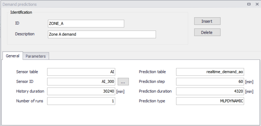
Figure: Example - Demand predictions data input