2D Weirs

In MIKE+, the 2D weir is used to represent a structure that raises the water level upstream and regulates flow downstream. E.g. a low dam.

A weir is located with a cross (line) section where the total discharge across the cross section is calculated using empirical formulas and distributed along the cross section. In the numerical calculations the weir cross section is defined as a section of element faces (from the 2D domain mesh/grid which is treated as an internal discharge boundary).

Insert

This option enables the user to manually digitise along the path of the weir in the 2D domain.

Steps to digitise:

• Click on the "Insert" button at the top of the 2D weir table
• Left click along the width of the weir in the 2D domain. Tip: right click to undo the previous graphical point
• Double click to complete the digitisation.

Insert from File

Import the path of the weir from an external source such as a Shape, XYZ or tab file.

The text file format is two space separated floats (real numbers) for the x- and y-coordinate on separate lines for each of the points.

Location and Levels

Weirs are located in the 2D domain with a cross (line) section specified as a list of points in the location and levels table (a minimum of two points required). The section is composed of a sequence of line segments. The line segments are straight lines between two successive points (see Figure 3.44).

Info

The faces defining the line section for the weir will be listed in the 2D simulation log file.

Insert, delete, manually edit values or change the order of the digitised points as needed.

Geometry

The geometrical layout of the weir must be specified.

A range of formulas are available to be applied to each weir structure:

• Broad Crested Weir Formula
• Villemonte Formula
• Honma Formula

Broad Crested Weir Formula

For a broad crested weir the geometrical shape of the active flow area of the weir needs to be defined. The geometry is defined as a Level-width relationship, where the Level/Width table defines the weir shape as a set of corresponding set of levels and flow widths. Values in the level column must be continuous, increasing values.

 

Figure: Setup definition of contracted weir

 

Figure: Definition sketch of broad crested weir geometry

Levels are defined relative to the datum (starting from the crest or sill level, upwards). A datum value for the weir may be used to shift the levels by a constant amount. This is typically used if the weir geometry has been surveyed with respect to a local benchmark.

The standard formulations for flow over a broad crested weir are established on the basis of the weir geometry and the specified head loss and calibration coefficients (see Head Loss Factors). These formulations assume a hydrostatic pressure distribution on the weir crests. Different algorithms are used for drowned flow and free overflow, with an automatic switching between the two.

The energy loss over a weir is given by:

(3.17)   

where \(z_{t}\) is the total head loss coefficient and \(V_{s}\) is the mean cross sectional velocity at the structure. The total head loss coefficient, \(z_{t}\) is composed of entrance, \(z_{1}\), and exit, \(z_{2}\), loss coefficients. The coefficients are generally related to the input parameters for inflow, \(z_{in}\), and outflow, \(z_{out}\), and the changes in velocity, V and area A.

(3.18)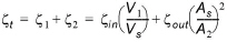   

where suffix '1' and '2' represents velocity and area on the inflow and outflow side of the structure respectively, and 's' represents the velocity and area in the structure itself. However, in the present implementation, upstream and downstream cross sections are not extracted and accordingly, tabulated relations on cross section areas as a function of water levels are not known. Instead, upstream and downstream areas are set to a large number resulting in a full loss contribution from the head loss factors defined

(3.19)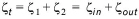   

Care must be taken when selecting loss coefficients, particularly in situations where both subcritical and supercritical flow conditions occur. When flow conditions change from subcritical to supercritical (or the Froude number, FR, becomes greater than 1), the loss coefficients \(z_{in}\) and \(z_{out}\) are modified:

• If FR > 1 for upstream conditions, then \(z_{in} = z_{in}/2\)
• If FR > 1 for downstream conditions, then \(z_{out} = z_{out}/2\)

The critical flows are multiplied by the critical flow correction factor, \(a_{c}\), specified as the free overflow head loss factor. Typically, a value of 1.0 is used.

Villemonte Formula

 

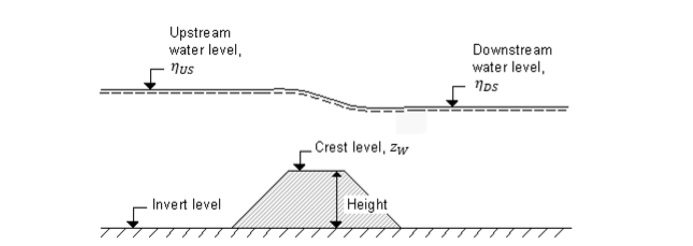
Figure: Definition sketch for Weir flow

For this type of weir the width, height and invert level for the weirs must be specified (figure above). The width is perpendicular to the flow direction. Typically, the invert level coincides with the overall datum. In addition, a weir coefficient and weir exponent must be specified.

This formula is based on a standard weir expression, reduced according to the Villemonte formula.

(3.20)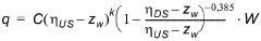   

where q is the discharge through the structure, w is the width, C is the weir coefficient, k is the weir exponential coefficient, \(h_{US}\) is the upstream water level, \(h_{DS}\) is the downstream water level and \(z_{w}\) is the weir level. The invert level is the lowest point in the inlet or outlet section respectively.

Honma Formula

For this type of weir the width and crest level for the weirs must be specified (see figure above). The crest level is taken with respect to the global datum. The width is perpendicular to the flow direction. In addition, a weir coefficient must be specified.

The Honma formula is expressed as:

(3.21)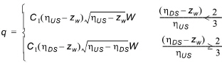   

where q is the discharge through the structure, W is the width, \(C_{1}\) and  are the two weir coefficients, \(h_{US}\) is the upstream water level, \(h_{DS}\) is the downstream water level and \(z_{w}\) is the weir level.

Attributes

The user can control which culverts are activated during the simulation using the "Apply" switch.

The parameters below define the weir characteristics.

Dampening Delta Depth

When the water level gradient across a structure is small the corresponding gradient of the discharge with respect to the water levels is large. This in turn may result in a very rapid flow response to minor changes in the water level upstream and downstream.

The dampening delta depth is the water level difference at which the discharge calculation is described by a linear variation. If the water level difference is below this value the discharge gradients are suppressed.

The default setting is 0.01 meter. If a structure shows oscillatory behaviour it is recommended to increase this value slightly.

Non-Return Flap

The following options are available:

• None: No valve regulation applies (flow is not regulated).
• Only left to right flow: Only flow in the positive flow direction is allowed. Valve regulation does not allow flow in the negative flow direction in which case the flow through the structure will be zero. The flow direction is positive when the flow occurs from the right of the line structure to the left, positioned at the first point and looking forward along the line section.
• Only Negative Flow: Only flow in the negative flow direction is allowed. Valve regulation does not allow flow in the positive flow direction in which case the flow through the structure will be zero.

 

Figure: Positive and Negative flow direction definition for weirs and culverts

Flow Distribution

The total discharge across the weir is calculated based on the mean water level in the real wet elements that directly neighbour the section of 2D mesh/grid faces that define the weir. For an irregular mesh, the mean level is calculated using the length of the element faces as the weighting factor. Real wet elements are elements where the water depth is larger than the wetting depth. The upstream water level is then the highest of the two water levels and the downstream water level the smallest.

The distribution of the calculated total discharge along the section faces can be specified in two ways

• Uniform
• Non-uniform.

When non-uniform distribution is selected the discharge will be distributed as it would have been in a uniform flow field with the Manning resistance law applied, i.e. is relative to \(h^{5/3}\), where h is the depth. This distribution is, in most cases, a good approximation. This does not apply if there are very large variations over the bathymetry or the geometry. The distribution of the discharge only includes the faces for with the element to the left and the right of the face is a real wet element. In no elements on the downstream side of the structure are real wet elements the distribution is determined based on the upstream information.

Note

For Composite structures (when multiple short culverts and/or weirs are located on the same faces) the distribution for the first structure is applied.

Head Loss Factors

The factors determining the energy loss occurring for flow through hydraulic structures. Head Loss Factors are only applied for a broad crested weir.

The following head loss factors can be defined (for positive and negative flow directions):

• Inflow (contraction loss)
• Outflow (expansion loss).

Calibration factors

Calibration factors can also be applied besides head losses.