Results Differences Tool
Introduction
The 'Result differences' tool is designed for comparing results from different variants of hydraulic network simulations, and report any significant difference of result. This may e.g. be used when comparing results from a former version of the model and results from a new version updated with the latest information from an asset management system. The tool allows you to:
-
Quickly identify locations where results differences are observed
-
Visualise and compare results at the identified locations, to verify whether the differences are acceptable or not.
The 'Result differences' tool is accessible from the 'Results' tab in the ribbon. It is not necessary to have a model database opened for using the tool.
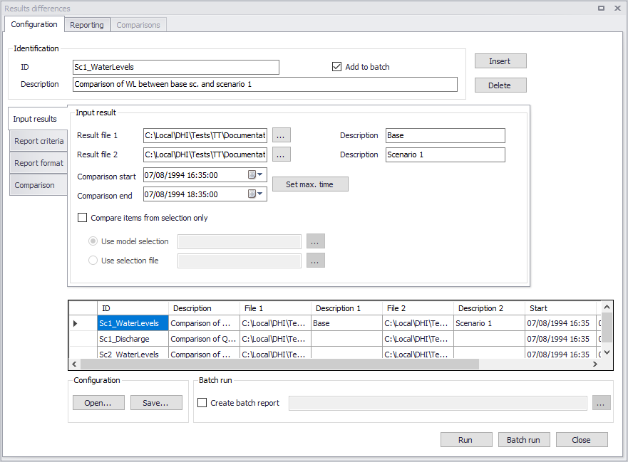
Figure: The Results differences tool
Note
If one of the two compared result files contains a network with pipes merged using the 'Network simplification' tool, the comparison can take into account the simplification information, in order to compare results in the original pipes and the merged pipe even though they have a different ID. This requires that the model database with the simplified network, which stores simplification information (relationships between IDs of original and merged pipes), is opened when the 'Results differences' tool is executed.
Running the tool
The tool can handle one or multiple comparison jobs. One comparison job can compare only one result item (water level, discharge, etc.) between two result files. If more result files and/or more result items should be compared, then extra comparison jobs must be used. Comparison jobs are added or removed using the 'Insert' and 'Delete' buttons at the top, and are listed in the table at the bottom of the dialog.
To start using the tool, a first comparison job must be inserted.
Each comparison job is given an ID, and can optionally contain a description, specified at the top of the dialog.
The 'Run' button will run only the active comparison job from the table.
The 'Batch run' button will run all the comparison jobs which have their option 'Add to batch' active.
Each comparison job gets its own report, but for a batch run it is also possible to get an overview report for the entire batch run. This is enabled by ticking the option 'Create batch report' and selecting the path and name of the batch report file. The batch report shows the number of time series for which the criteria were exceeded during the comparison.
Once the tool has been configured, it is possible to save its configuration to a file using the 'Save…' button for later re-use. This configuration can later be loaded again using the 'Open…' button, or can be used to execute the tool from a command line.
Input results
The 'Input results' tab contains information controlling the selection of time series to be compared.
Result files 1 and 2
These are the paths to the result files selected for the comparison. Press the '…' buttons to select the files. The supported file types are:
- .res1d (MIKE 1D result files from collection systems and/or river networks, excluding catchments results)
- .res (Water Distribution / EPANET result files)
- .out (SWMM result files).
Result file 1 and Result file 2 must be of the same file type for a given comparison job. Other file types (typically .resx, .msxr and .whr) cannot be compared in this tool.
The comparison is done based on the network element ID, i.e. nodes or pipes / rivers should have the same ID in the two result files in order to be compared.
Result file 1 is the reference file. The two result files don't have to store results at the same date and time: when they differ, the results from the result file 2 are linearly interpolated to match the dates and times in result file 1.
Descriptions
Optional descriptions for the result file 1 and result file 2, respectively.
Comparison start and end
The time interval for which the comparison is executed can be set here. It is possible to execute the comparison for a limited period, shorter than the complete overlap between the files.
The 'Set max. time' button can be used to set the common time interval for the two result files as the comparison period.
Compare items from selection only
By default, the tool will compare all result time series for locations found in the two compared result files.
It is also possible to reduce the number of time series being compared by activating the option 'Compare items from selection only' and choosing a selection containing the list of items to be compared. Two options are available to choose the selection:
- Use model selection: this option is used to pick a selection defined in the 'Selection manager', accessible from the Map tab in the ribbon. This option requires that a model database is opened, to access the list of selections. When no model database is opened, this option is therefore disabled.
- Use selection file: this option is used to pick a selection defined in a text file. This text file can be created by saving a selection defined in the 'Selection manager', accessible from the Map tab in the ribbon. This option is always available, even if no model database is opened.
Report criteria
The 'Report criteria' tab contains information controlling the reported differences in the report.
Result item
Only one result item can be selected for a given comparison job. The list of available compared items depends on the result files type. For .res1d result files, the possible compared items are:
- Discharge: this result item is not available at nodes, and will therefore be compared on links only.
- Water level: this result item is available in both nodes and links.
- Flow velocity: this result item is not available in nodes nor in structure reaches, and will therefore be compared on regular links only.
- Volume: this result item is available in both nodes and links.
Note that the 'Volume' result item is not included by default in result files and must be added manually before running the simulation.
For .res result files, the possible compared items are:
- Flow: this result item is not available at junctions, and will therefore be compared on links only.
- Velocity: this result item is not available at junctions, and will therefore be compared on links only.
- Pressure: this result item is compared in junctions and tanks.
- Head: this result item is compared in junctions and tanks.
- Water quality: this result item is compared in nodes and links.
- Water demand: this result item is compared in junctions and tanks.
For .out result files, the possible compared items are:
- Discharge: this result item is not available at nodes, and will therefore be compared on links only.
- Water depth: this result item is available in both nodes and links.
- Flow velocity: this result item is not available in nodes, and will therefore be compared on links only.
- Volume: this result item is available in both nodes (result item called 'Node volume stored & ponded') and links ('Link volume').
Each option represents the instantaneous value of the result item in the compared calculation point.
Acceptance criteria
It is possible to select and combine various criteria for the comparison. In general, the result computed for the individual criterion is based on the absolute difference between the two time series being compared. This means that the result indicates if the time series deviate, but the result does not indicate which time series has e.g. the largest maximum value.
In an ideal case, when the two time series are identical, the value computed by each criterion should be zero. The only exception is the 'Confidence band' criterion, which results in a value of 100 when comparing two identical time series. In practice, when comparing two different time series, values close to zero (or close to 100 for 'Confidence band') indicate a good similarity. On the contrary, if the computed values are significantly far from zero (or from 100), the similarity of the two time series is weak.
When a criteria is selected, it is included in the comparison process. If the specified criteria is fulfilled (e.g. Peak error \<= 2%), then the difference between the two time series is considered acceptable. When one or more criteria is not fulfilled, the comparison is "rejected" and the time series is listed in the report.
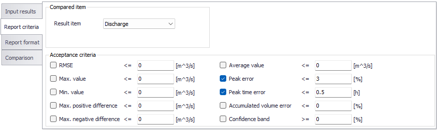
Figure: The Report criteria tab
If the computed value indicates that the time series deviate, then a more detailed inspection of the time series is recommended to determine the importance of the difference.
The criteria are described below in more details. In these descriptions, \(y_{1}\) always refers to the instantaneous value of the time series from Result File 1, while \(y_{2}\) refers to the value from Result File 2.
Root Mean Square Error (RMSE)
The Root Mean Square Error (RMSE) criterion can be applied as a measure for the magnitude of the deviation between the two time series over the period being investigated.
(18.1) 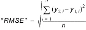
The values for the second time series (Result File 2) will be linearly interpolated to get values at the date and times matching the Result File 1.
Maximum value
The criterion provides a value for the difference in maximum values found in the two compared time series.
(18.2) 
It should be noticed that the maximum value found in the two time series does not necessarily occur at the same point in time in the two series.
Minimum value
The criterion provides a value for the difference in minimum values found in the two compared time series.
(18.3) 
It should be noticed that the minimum value found in the two time series does not necessarily occur at the same point in time in the two series.
Maximum positive difference
This criterion computes a value indicating how much the first time series (Result File 1) is above the second time series at the point in time where this difference has its maximum.
(18.4) 
The values for the second time series (Result File 2) will be linearly interpolated to get values at the date and times matching the Result File 1.
Maximum negative difference
This criterion computes a value indicating how much the first time series (Result File 1) is below the second time series at the point in time where this difference has its maximum.
(18.5) 
The values for the second time series (Result File 2) will be linearly interpolated to get values at the date and times matching the Result File 1.
Average value
The average value is computed for both time series. Each value is given weight according to the actual time step. Values are assumed valid for the time interval since the previous value. As a consequence, the first value is ignored.
(18.6) 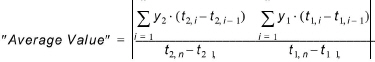
Peak error
This criterion computes a value for the relative error for the maximum values.
(18.7) 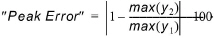
It should be noticed that the maximum value found in the two time series does not necessarily occur at the same point in time in the two series.
Peak time error
This criterion indicates how far in time the two maximum values a located away from each other. This criterion can be used to clarify if the criteria 'Max Value' and 'Peak Error' actually compare the same event.
(18.8) 
Accumulated volume error
This criterion is only available when comparing a discharge or water demand result item. It computes the deviation (in percentage) of accumulated volume through nodes and grid points from the discharge time series.
(18.9) 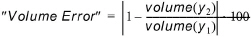
Where Volume(y) is the accumulated volume in a calculation point computed from the discharge time series:
(18.10) 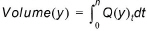
Confidence band
The purpose of this criterion is to verify that two time series are identical at all points. It is accepted that the two time series are shifted in time by maximum one time step and a tolerance (dx) is accepted.
(18.11) 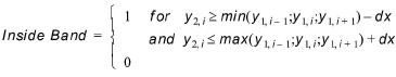
(18.12) 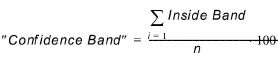
The values for the second time series (Result File 2) will be linearly interpolated to get values at the date and times matching the Result File 1. Tolerance (dx) is set to 0.01.
Note
For this criterion the ideal value is not zero but 100.
Note
When a model database is opened, the criteria's units are controlled by the selected unit system in the model setup. If no model database is opened, the unit is controlled by the 'Preferred unit system': see File Menu for more information.
Report format
The 'Report format' tab contains information controlling the format of the reported differences, for the active comparison job.
Report
This is the path to the report file, for the active comparison job. The report is saved to a *.htm file, which can be opened in a web browser.
Comment
An optional description of the active comparison job, which will appear in the report.
Report differences only for gidpoints where criteria are exceeded
By default, this option is active and the report will list only the locations where the acceptance criteria are not fulfilled (i.e. where differences are significant). If this option is unselected, all locations will be reported, therefore also providing the comparison values for the locations where the differences are small.
Create shape file with differences where criteria are exceeded
When this option is selected, the locations where the acceptance criteria are not fulfilled (i.e. where differences are significant) are saved to a shape file. This makes it easy to visualize the locations of significant differences on a map.
Two shape files can be created:
- A point shape file storing nodes locations.
- A line shape file storing links locations.
The specified file name is used by the lines shape file. The nodes shape file has the same file name but with a suffix '_Nodes'.
If the location of the link or node on the map differs between the two result files, the shape file will show the location from the first result file.
Graphics
This option controls if time series plots are included in the report or not. Three options are available:
- Don't include time series: no time series is added to the report.
- Include time series without difference: for the reported locations, a time series plot will show the superimposed time series from the two result files.
- Include time series with difference: for the reported locations, a time series plot will show the superimposed time series from the two result files plus an extra time series showing the differences between the two files, on a secondary Y-axis.
Note
Including time series in the report may significantly increase the results comparison time as well as the report file size, depending on the number of included graphics.
Comparison
The 'Comparison' tab contains information controlling optional additional comparison plots, which can be provided after running the comparison job.
The following additional plots can be activated.
Scatter plot
The scatter graph is an analysis plot where the horizontal axis is the magnitude of the results from the first file and the vertical axis is the magnitude of the results from the second file. At each time step saved in the first result file, the result from the second file is interpolated so that it can be plotted as an X,Y point on the graph. If the model and data are in perfect match, then the point is plotted on a 45-degree line. If the result file 1 is low by comparison with the result file 2, then the point will be plotted above the 45-degree line.
The red line in the scatter plot is the line of best fit. The value 'a' is the slope of the line and value 'b' is the Y-axis intercept.
The scatter plot visually shows if there is high or low behavior in specific value ranges, and also the width of the scatter gives a qualitative estimate of the amount of variability at a given value range. The analysis therefore allows the modeller to observe where the bias occurs in general areas of the modeled behavior.
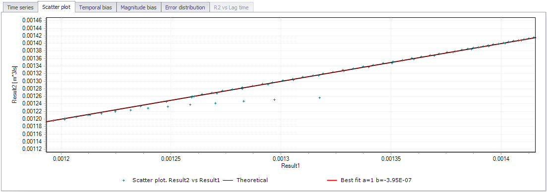
Figure: The Scatter plot
Temporal bias
The temporal bias is defined as the difference between the two result files at the same point in time, expressed as (Result file 2 - Result file 1). This plot indicates when this temporal bias occurs, and if it is a regular or random occurrence. This plot tends to show if there are certain time periods where errors occur. If there are multiple instances of the same behavior, then it is not due to an isolated event and is something which repeats.
A line of best fit is calculated, and if the slope on the line is zero (i.e. the line of best fit is parallel to the horizontal axis), then there is no trend of bias in the comparison. In the case where the slope is zero but the Y-intercept is non-zero, then there is probably a baseflow error.
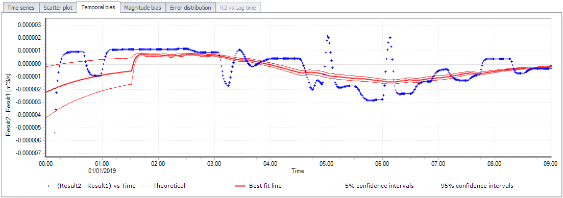
Figure: The Temporal bias plot
When activating the temporal bias plot, a time interval must be specified. The temporal bias plot is divided into a number of time periods, and the values in the time interval are used as a population to calculate mean and 5% and 95% confidence intervals. The confidence intervals are based on the assumption that the error is normally distributed.
Magnitude bias
The magnitude residual plot is like the scatter graph but normalized to a horizontal axis. By plotting the difference between the two files on the vertical axis and the average of the two files on the horizontal axis, the line of best fit becomes a horizontal line intercepting the Y-axis at zero. Hence this plot shows more clearly the width of the scatter at certain values ranges, and will signal wide errors at certain hydraulic conditions or when certain thresholds are exceeded.
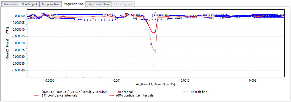
Figure: The Magnitude bias plot
When activating the magnitude bias plot, a number of intervals must be specified.
Error distribution
This plot does not perform any analysis, but it gives an indication of where the two result files diverge on a percentage basis. The error distribution value yi is expressed like this:
(18.13) 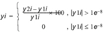
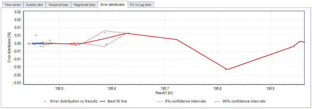
Figure: The Error distribution plot
When activating the error distribution plot, a number of intervals must be specified.
R2 vs. Lag time
This plot is specifically designed to analyze if there are lags in one of the result files which would otherwise provide a good fit. The analysis is therefore very useful for determining if there are travel time errors.
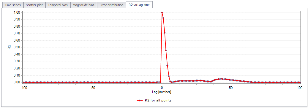
Figure: The R2 vs Lag time plot
When activating the R2 vs Lag time plot, a number of time lags to be analysed as well as the lag duration must be specified. The tool then shifts one time series both forward and backwards in time compared to the original position, and calculates the coefficient of determination \(R^{2}\) for each position. The plot produced is a plot of number of lags on the horizontal axis (both negative and positive) and the coefficient of determination \(R^{2}\) on the vertical axis. The plot can be used to determine if there are fundamental time shifts in the information.
Note
Activating the R2 vs Lag time plot requires much more computational resources than for the other plots. Therefore, when this plot is included in the analysis, the computational time may increase significantly.
Reporting
After running a single comparison job or a batch run, the 'Reporting' tab is opened
Reports
The upper table shows a list of the report files generated during the run. Each file can be opened using the 'Open' button.
Run status
The different steps of the comparison are listed here, along with possible errors encountered during the run.
Comparisons
The 'Comparisons' tab shows the result of the comparison job.
Location table
The table in the upper left corner shows the list of locations where time series have been compared. The active record in this table selects at which location the criteria values are reported on the right, and at which location the time series are plotted at the bottom.
The table contains three columns:
- Type: the network element type (link, node, structure type).
- ID: the ID of the network element.
- Chainage: the chainage / distance of the calculation point along its link. Not applicable for nodes.
Two types of filters are available above the table, to help searching an item by reducing the displayed list:
- A Search field: type here the expected text to search in the ID column. Press the 'Clear' button to clear this filter.
- A type selection: use the list on the right above the table, to show only the locations for a given type (Node, pump, orifice, etc.).
ID
In the 'General' group, the ID shows the ID of the comparison job being displayed.
Result item
The 'Result item' shows the item being compared in the displayed comparison job
Show time series of differences
By default, the 'Time series' tab shows the superimposed time series from the two compared result files, only. When this option is active, it also shows an extra time series plotting the difference between the two, on the secondary Y-axis.
Show rejected gridpoints only
By default, all locations are shown in the location table on the left. When this option is active, the table shows only the locations where one or more criteria are not fulfilled.
Result statistics
This group shows the result statistics values for the active location in the location table (upper left table), when they have been selected as acceptance criteria for the comparison.
Comparison criteria
This group shows the calculated comparison values for the active location in the location table (upper left table), when they have been selected as acceptance criteria for the comparison.
It also shows the coefficient of determination R2, also known as Nash-Sutcliffe efficiency, that measures how well the result values in File 1 and File 2 match. This criterion is widely used to evaluate model performance in hydrological modelling. It ranges from minus infinity to 1 with larger values indicating a better fit. An important special case is R2 = 0, which can be obtained if the mean value from result file 1 equals the mean value from result file 2, indicating that the average of the result file 1's values in this case is as good a predictor as the result file 2. Thus, one would most likely require that R2 > 0 for the two files to be fit. The R2 criterion measures the one-to-one relationship between the two files' values, and hence it is sensitive to bias and proportional effects. It should be emphasized that R2 is based on the sum of squared residuals, and hence provides the same information on goodness-of-fit as the RMSE measure.
(18.14) 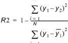
Where  is the mean value of the time series from result file 1.
The values for the result file 2 are linearly interpolated to get values at the same date and times as in result file 1. The calculation of this criterion is valid only when the result file 1 contains a constant time step.
Plots
The lower part of the dialog shows time series plots, for the active location in the location table (upper left table).
The 'Time series' tab is always active and shows the superimposed time series from the two compared result files. When 'Show time series of differences' is active, it also shows an extra time series plotting the difference between the two, on the secondary Y-axis.
The other tabs show optional extra plots, when they have been activated in the comparison configuration before the run.
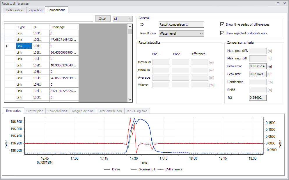
Figure: Results of the comparison job
Running the tool from command lines
When working with numerical models and their results, you often utilize the MIKE+ editor to access all the tools, including the 'Results differences' tool. However, there are times when it is required to compare result files in an automated way without opening the tool in the user interface.
The MIKE+ executables enable you to execute some tools without opening the editor, through command lines. It is possible to run the 'Results differences' tool in this manner, assuming you have prepared the comparison configuration file beforehand in MIKE+.
Start by locating the MIKE+ executable named DHI.MIKEPlus.ToolShell.exe in the installation folder. From a command prompt, type the command below to access the list of supported tools, replacing the … characters by the actual path to the file:
The format of the command for running the 'Results differences' tool is:
Where [Configuration file] is the path to the *.xml configuration file.
The only option available is: -c [Comparison ID]. This option may be used to execute only a specific comparison job from the list of jobs in the selected configuration file. When this option is not included, all comparisons added to the batch will be executed.