Time Series Plot

Time series can both be input time series or time series taken from result files.

In this section, the focus is on displaying time series from result files. Start by loading a result file into MIKE+, see Chapter 20.3 Loading Results.

There are basically two ways to create new time series plots:

• From a list of files and locations, using the ‘Create time series plot’ tool. This tool is only relevant for 1D result files and dfs0 time series files. This tool is accessed from the 'Time series plot' button in the 'Results' tab in the ribbon, or from a right-click on a result file or one of its result items. In this dialog:
  • Choose the result file, result item and locations to plot from the list. Use the filters to search through the potentially long list of available locations, to filter on ID and/or chainages (chainage filtering being available only for link results from .res1d result files). One may also use a selection list (saved in the ‘Selection manager’) or the active selection, to select all items from the selected list.
  • Select between ‘Create new plot’ and ‘Add to existing’ options and click on the ‘OK’ button.
• By picking a location on a map, using the ‘TS from map’ tool. This tool is accessed from the 'TS from map' button in the 'Results' tab in the ribbon The ‘Add time series from map’ dialog appears, wherein one specifies:
  • Source file
  • Source group
  • Source item
  • Specify whether to ‘Create a new plot’ or to ‘Add to existing’, click on the 'OK' button and finally select the corresponding model item on the map for which to plot time series results. To include multiple locations in the plot, either hold the 'Ctrl' key down while clicking on the map, or continue to click locations once the plot has been created. To stop adding more time series when clicking on the map, deactivate the 'TS from map' button in the ribbon.

 

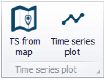
Figure: Time series plot tools on the Results ribbon

 

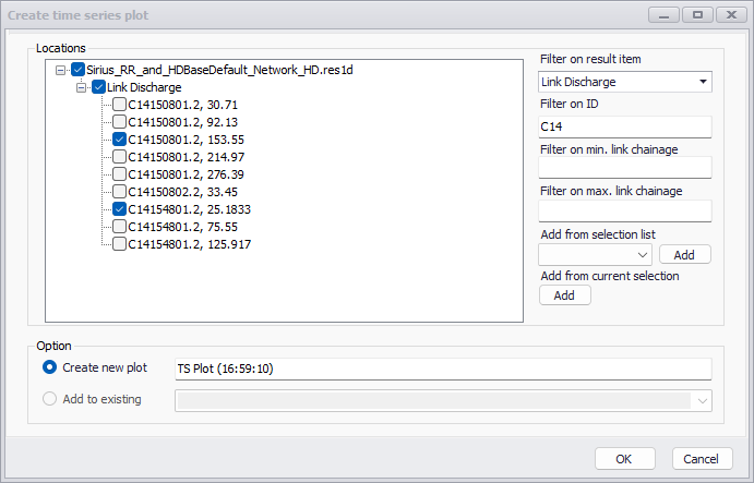
Figure: ‘Create time series plot’ window, showing the full list of result locations

 

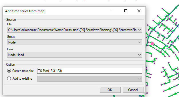
Figure: The ‘TS from map’ tool, to select result locations from the map

Once a time series plot is created, additional result time series can be added to the plot in various ways:

• Right-click in the table of content of the time series plot and select 'Add items
• Use the 'TS from map' tool with the option to add the new items to an existing plot
• Use the ‘Create time series plot’ tool with the option to add the new items to an existing plot
• Drag a result item from the 'Results' tree (click the '+' box to the left of a result file name to expand its list of loaded result items) and drop it in the table of content of the time series plot
• Add result items from another time series plot, using the Copy / Cut / Paste options in the context menu of the table of content.

 

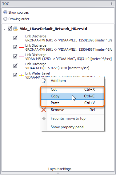
Figure: Options to copy and paste time series from one plot to another

Note

In the 'Create time series plot' window, filters are used to hide some items in the list but do not unselect them, i.e. a location can be selected and later become hidden using a filter, but will still be plotted when clicking 'OK'. The buttons 'Add from selection list' and 'Add from current selection' will tick all items from the selection, for all result files and result items which are visible, excluding those which are hidden due to filters.

Data series format

To customize the appearance of TS plot data series, right-click on a data series and activate the ‘Show property panel’ option from the local context menu.

Options for configuring data series appearance include customizing line color and style, adding markers, and changing marker styles and size.

 

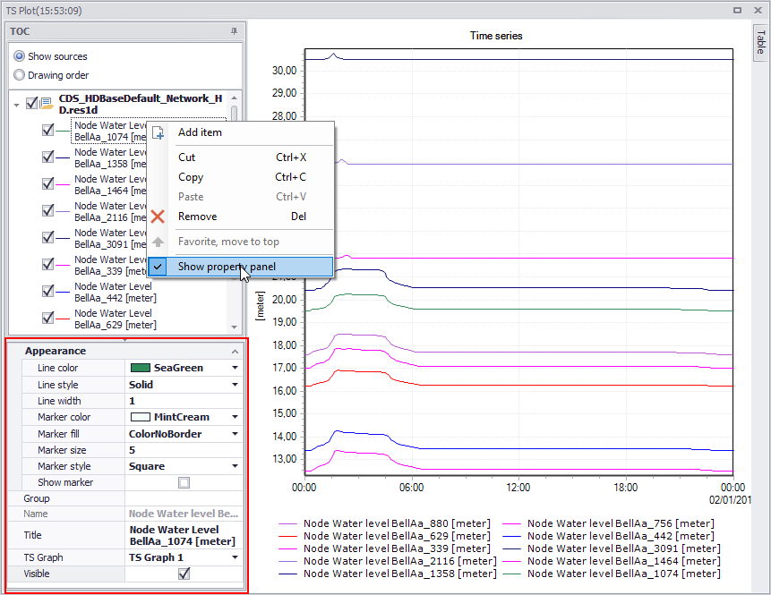
Figure: Customize the appearance of TS Plot data series via the Property panel

Context menu

Right-click on the time series plot to access options to control the zoom level, save the time series plot, copy data or export to an image file.

'Zoom in' lets you draw a rectangle on the plot to select the area to zoom to. While drawing a rectangle, dragging to draw a horizontal line will display arrows to zoom along the horizontal axis only, keeping the vertical axis unchanged. Similarly, dragging to draw a vertical line will zoom along the vertical axis only. 'Zoom to full extent' brings you back to the full view of visible time series. Note that additional options are available to control the zoom options:

• Hold down the Shift key, to zoom in
• Scroll with the mouse wheel to zoom in or out
• Hold down the Ctrl key to pan.

The 'Bookmarks' menu opens the bookmarks manager which can save and restore zoom extents. It contains the following options:

• Add: adds a new bookmark, saving the current time extent shown on the plot
• Zoom to: zooms to the time period saved for the bookmark selected in the left list
• Rename: renames the bookmark selected in the left list
• Remove: removes the bookmark selected in the left list
• Close: closes the bookmarks manager.

Note

Bookmarks only save the time extent (X axis), but not the extent on the vertical axis, and can therefore be applied to any plots even if they don't all have similar ranges of Y values.

 

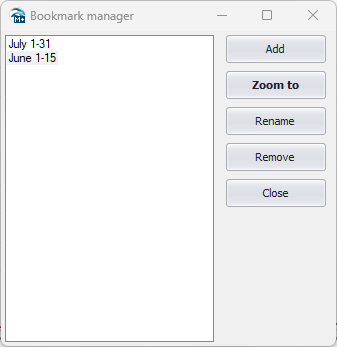
Figure: The bookmark manager from the time series plots

'Sync zoom in all plots' allows to apply the time extent (X axis) from one plot to all other opened time series plots. Two options are available:

• This time only: this option applies the time window from the active plot (from which the option is activated) to all other opened time series plots. Later changes to the zoom level in any plot have no automatic effect on the other plots.
• Always: this enables an automatic synchronization of the time window in all opened time series plots. Any change to the zoom level along the X axis in any plot also applies instantaneously to the other plots. Click again this 'Always' option to turn off this automatic synchronization.

'Save to plots manager' will save the time series content (list of time series locations and display settings) to the 'Plots' panel. The time series plot will initially be added to the active folder from this panel. See 'Plots Management' chapter for more information on options to save and manage results windows.

'Copy plot to clipboard' will copy the plot as an image in memory, to be pasted in another program. 'Copy data to clipboard' will copy the time series values in memory, to be pasted in another program.

'Save data to .dfs0 file' will save the time series to an external .dfs0 file, which can later be e.g. used as boundary condition for a future simulation or loaded as a result file in the 'Results' tree.

 

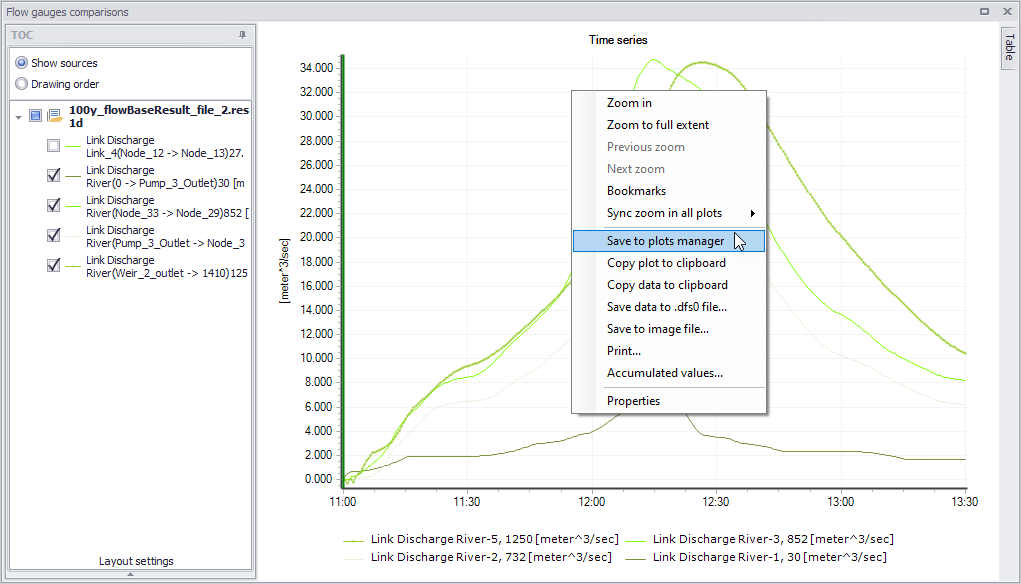
Figure: Context menu of the time series plot

When a time series has a unit which can be accumulated over time (e.g. discharge), the context menu offers an 'Accumulated values' option, which will compute the accumulated values over a given period of time. Three options are available to define this period: entire period, zoom extent, or custom period. In the latter case, the start and end date and time of the period can be customised.

After selecting the period, press the 'Compute' button to view the results of the accumulated values over the selected period, for each time series item.

 

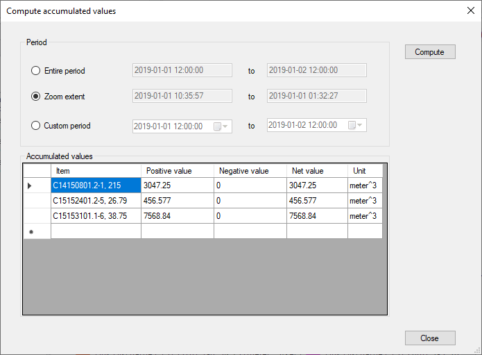
Figure: Compute accumulated values from time series

For each time series, the table shows :

• The positive value, which is the accumulated result of the positive values from the time series
• The negative value, which is the accumulated result of the negative values from the time series
• The net value, which is the accumulated result of all values from the time series.

Note

These accumulated values are computed from the time series stored in the result files, and therefore the accuracy of the accumulated values depends on the saving frequency of the results. If the saving frequency is low (i.e. long time step between two saved results), then the available results will not reflect significant variations of results between two saved time steps, and the calculated accumulated values may deviate from the actual simulated accumulated values.

The context menu also offers a 'Properties' option to control the layout and the symbology of the time series plot.