2D Dikes
In MIKE+, 2D dikes represent a natural or artificially constructed elongated ridge (levee, embankment, stopbank, etc) that can be used to regulate water levels. These often run parallel to the course of a channel/river in its floodplain or along low-lying coastlines.
Insert
This option enables the user to manually digitise along the path of the dike in the 2D domain.
Steps to digitise:
- Click on the "Insert" button at the top of the 2D dikes table
- Left click along the path of the dike in the 2D domain. Tip: right click to undo the previous graphical point
- Double click to complete the digitisation.
Insert from File
Import the path of the dike from an external source such as a Shape (.shp), XYZ (.xyz) or tab (.tab) file.
The format for XYZ files is three space separated floats (real numbers) for the x- and y-coordinate and the crest level on separate lines for each of the points.
When importing a path from a file, ensure that the map projection (Longitude/Latitude, UTM, etc.) correlates with the MIKE+ project projection.
For shape files, if the input file is a 3D shape file (containing crest levels in the lines geometry), then all the lines from the file are imported simultaneously as separate dikes, and the crest levels are also imported from the file. For regular shape files, each file should contain a single line corresponding to a single dike.
Location and Levels
Every dike digitised or imported will have georeferenced points (x and y coordinates) which together make up a polyline along the path of the dike. A minimum of two points is required. The polyline defines the width of the dike perpendicular to the flow direction. The polyline is composed of a sequence of line segments. The line segments are straight lines between two successive points. The polyline (cross section) in the numerical calculations is defined as a section of element faces. The face is included in the section when the line between the two element centres of the faces crosses one of the line segments (see Figure 3.44).
Info
The faces defining the line section for the dike will be listed in the logfile.
Insert, delete, manually edit values or change the order of the digitised points as needed.
The geometry of a dike is defined as shown below where the Z values refer to the elevation / crest level of the dike.
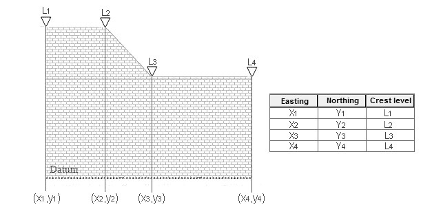
Figure: Definition sketch of spatial varying dike geometry
Attributes
Control which dikes are activated during the simulation using the "Apply" switch.
The parameters below define the dike characteristics.
Dampening Delta Depth
When the water level gradient across a structure is small, the corresponding gradient of the discharge with respect to the water levels is large. This in turn may result in a very rapid flow response to minor changes in the water level upstream and downstream. As a way of controlling this effect, a dampening delta depth has been introduced. The critical water level difference defines the water level difference below which the discharge gradients are suppressed. The default setting is 0.01 meter. If a structure shows oscillatory behaviour it is recommended to increase this value slightly.
Weir Coefficient
A dike is defined as a cross section and in the numerical calculations the cross section is defined as a section of element faces which is treated as an internal discharge boundary. (However, the flux contribution to the continuity equation is corrected to secure mass conservation). The discharge across each face in the section is calculated using an empirical formula. The discharge over an element face with associated width, is calculated based on the water level in the elements to the left and right of the face. The upstream water level is then the highest of the two water levels and the downstream the smallest.
The flow, Q, over a section of the dike corresponding to an element face with the length (width), w, is based on a standard weir expression, reduced according to the Villemonte formula :
(3.12) 
where Q is discharge through the structure, w is the local width (cell face width), C is discharge coefficient, \(H_{us}\) is upstream water level, \(H_{ds}\) is downstream water level and \(H_{w}\) is the crest level taken with respect to the global datum.
The default value of the weir coefficient is 1.838.
Figure: Definition sketch for Dike Flow
Relative Change to Crest Level
The crest level relative change represents a change of the dike's crest level during the simulation, which is expressed as a relative depth compared to the initial crest level. It can be specified as:
- None
- Uniform
- Varying along dike
- Varying along dike and in time.
None
The crest level does not change and the original z levels defined for the dike are used.
Uniform
The crest level is defined by a specific value specified as an input (in m).
Varying along dike
The crest level is predefined for the dike in an external .dfs1 file. Browse to a file already created, edit a file or create a new file (the MIKE Zero interface is opened).
Varying along dike and in time
The crest level varying in time is predefined for the dike in an external .dfs1 file. Browse to a file already created, edit a file or create a new file (the MIKE Zero interface is opened).
For the external .dfs1 file, the number of grid points needs to correspond to the number of points, which is used to define the location of the dike. The data must cover the complete simulation period. The time step of the input data file does not however have to be the same as the time step of the hydrodynamic simulation. A linear interpolation will be applied if the time steps differ.