Cross Section Properties¶

The properties for cross sections are shown in the ‘Cross Section Properties’ panel on the upper right-hand side of the Cross Sections editor.

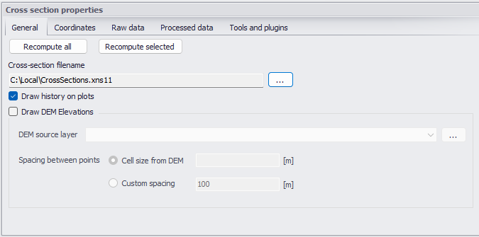
Figure: The Cross Section Properties panel on the Cross Sections editor

General¶

The General tab contains options and data which are relevant for all or part of all the cross sections.

Recompute all: The ‘Recompute all’ button recomputes processed data for all the cross sections.
Recompute selected: The ‘Recompute selected’ button recomputes processed data for only the selected cross sections (those having the ‘Select’ checkbox checked).
Cross-section filename: Cross sections are stored in a cross section file with the *.XNS11 file extension. Click the ‘…’ button to either select an existing file or to create a new one.
Draw history on plots: When this option is checked, watermarks are added as a history of previous cross sections drawn on the ‘Cross section plot’ and the ‘Processed data plot’. This feature allows comparison of multiple cross sections on a single scale.
Draw DEM elevations: When this option is checked, a green line is added on the 'Cross section plot', showing the elevations obtained from a selected DEM. This feature allows comparison of the active cross sections with e.g. a more detailed or more recent DEM. When this option is active, the following must be specified:
- DEM source layer: the input raster file containing the DEM data, from which the DEM plots will be obtained.
- Spacing between points: this is used to control the maximum spacing between points along the DEM line. By default, the maximum spacing is set to the cell size of the DEM raster. By changing to a custom spacing, any other custom value can be used.

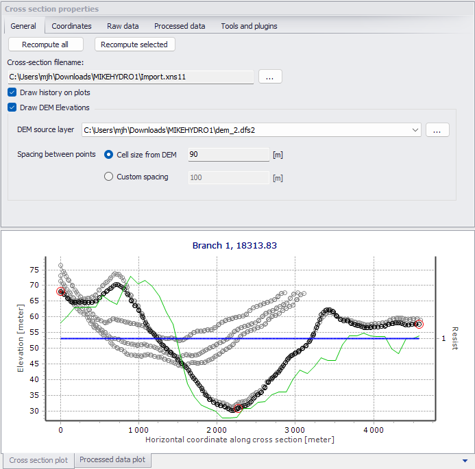
Figure: ‘Draw history on plots’ option shows previous cross sections, ‘Draw DEM elevations’ shows a green DEM line

Coordinates¶

One may customize the location of cross sections via the ‘Coordinates’ tab on the Cross Section Properties panel. The tab page tabulates vertices defining the location of the cross section (i.e. the red cross section polyline shown on the map). Each row describes a point defined by its X and Y coordinates expressed in the coordinate system used for features in the setup. These vertices do not have to match the list of points provided in the ‘Raw data’ tab.

The coordinates in the table must be sorted from the left side of the river (at the top of the table) towards the right side of the river (at the bottom of the table). The definition of the left and right sides of the river depends on the selected 'Flow direction' of the river branch. Refer to the Rivers definition description for more details.

When cross sections have been created from the Map view, the table is automatically filled with all vertices defining the location of the polyline and one point at the intersection with the branch.

When coordinates are provided in the table, the ‘Apply’ option can be activated. When applied, cross sections are displayed on the map based on the defined coordinates. Otherwise, the cross section is displayed perpendicular to the branch at the specified chainage, using the length calculated from the ‘Raw data’ tab.

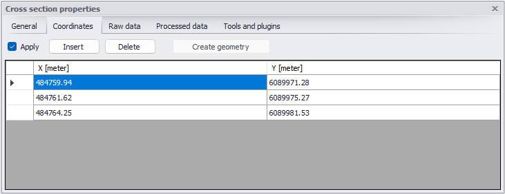
Figure: The Coordinates tab on the Cross Section Properties panel

Raw Data¶

The ‘Raw data’ tab tabulates points defining the topography of the river bed along the cross section. These points do not have to match the list of vertices provided in the ‘Coordinates’ tab.

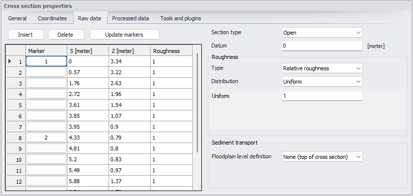
Figure: The Raw Data tab page on the Cross Section Properties panel

The ‘S’ column is the horizontal distance of each point along the cross section from the left end of the cross section. The points in the table must be sorted from the left side of the river (at the top of the table) towards the right side of the river (at the bottom of the table). The definition of the left and right sides of the river depends on the selected 'Flow direction' of the river. Refer to the Rivers definition description for more details.

The ‘Z’ column is the elevation of the points.

The ‘Insert’ button above the table can be used to insert a new line at the bottom of the table, while the ‘Delete‘ button can be used to delete the active line.

Markers may be assigned to points under the ‘Marker’ column of the table. Markers can be assigned in two ways. Click an element under the ‘Marker’ column, which opens a marker dialog as shown in the figure below from which a marker number may be defined for the selected point.

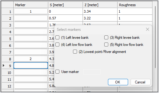
Figure: The Select Markers dialog

Alternatively, select a point on the cross section plot below the table, and press the marker number on the keyboard. Pressing the 'Ctrl' key and the marker number will remove the marker for the selected point on the cross section plot.

A number of markers may be defined:

Left and right levee banks (Markers 1 & 3): Defines the extent or the active part of the cross section used for calculations. Default placement of markers 1 and 3 is to apply marker 1 in the very first point in the raw data and marker 3 at the very last point of the raw data. Placing any of these markers at different locations will limit the extent of the active part of the cross section such that only the part of the cross section between markers 1 and 3 is included in the simulation (that is, Processed data are only calculated for cross section data between these markers).
Left and right low flow banks (Markers 4 & 5): Defines the extent of the low flow channel. The markers influence the calculation of the processed data. If defined, the section is internally divided into three major ‘slices’ at markers 4 and 5 positions and the resulting processed data for such a section is a sum of integration results of three sub-parts of the section instead of calculating a result from one single, large section.
- Additionally, markers 4 and 5 can be used to define the extent of the low flow channel which is used with the ‘High/low flow zones’ description of the resistance distribution in the raw cross section data.
Lowest point/River alignment (Marker 2): Marker 2 typically defines the lowest point of the river section, or the location of the intersection with the river line. Marker 2 settings do not affect the calculations. Instead, it is primarily used to place cross sections which have no coordinates defined along the river alignment. It is therefore recommended to define the correct position of marker 2 in all sections.
User marker: Any number above 7 may be used as a user marker. User markers do not impact the simulation results. They are an option for indicating a specific point in a cross section e.g. the location of a measurement gauge.

Note

Marker locations must be defined such that marker 1 is defined to the left of marker 3 in the raw data table.

Update Markers¶

This button automatically updates markers 1, 2 and 3 locations in the current cross section, which are at the left end point, lowest point, and right end point, respectively.

Section Type¶

The type of cross section is set here. Four options are available:

Open section: Typical setting for river cross sections.
Closed irregular: Closed sections with arbitrary shape.
Closed circular: Closed circular section shape where the geometry is only defined by the diameter.
Closed rectangular: Closed rectangular section shape where the geometry is only defined by the width and height.

Datum¶

A datum value may be entered here. The datum is normally used for adjusting the levels of the cross sections such that they conform to a specific reference datum in the model area. The datum value is added to all elevations in the ‘Raw data’ tab. The datum is also used for circular and rectangular sections to set the elevation of the bottom level of the cross section.

Roughness Type¶

There are various options for defining the desired type of roughness method for cross sections. The following types are available:

Relative roughness: The resistance/roughness is given relative to the roughness number specified in the ‘Bed roughness’ editor. The roughness value specified in the cross section for this roughness type is therefore a coefficient. A coefficient higher than 1 will increase the actual roughness of the river bed, whereas a coefficient lower than 1 will decrease the actual roughness. So when the roughness type is Manning (M) in the 'Bed roughness' editor, then the Manning's M value is divided by this coefficient. When the resistance type is Manning (n), then the Manning's n value is multiplied by this coefficient.
Manning’s n: The roughness number is specified as Manning’s n in the unit s/m(1/3).
Manning’s M: The roughness number is specified as Manning’s M in the unit m(1/3)/s (Manning’s M = 1/Manning’s n).
Chezy number: The roughness number is specified as Chezy number in the unit m(1/2)/s.
Darcy-Weisbach (k): The roughness is specified in the form of an equivalent grain diameter.

Note

Roughness numbers have to be defined in the ‘Bed roughness’ editor, as a global value and eventually local values. However, if absolute roughness numbers are defined in one or more cross sections as either Manning’s n, Manning’s M or Chezy number, then these numbers will have first priority and overrule any roughness values defined in the ‘Bed roughness’ editor.

Roughness Distribution¶

The distribution type defines the description of the transversal roughness across the cross section. Three options are available:

Uniform: A single roughness number will be applied uniformly throughout the cross section.
High/Low flow zones: Three roughness numbers are to be specified. The ‘Left high flow’ number applies between markers 1 and 4, the ‘Right high flow’ number applies between markers 5 and 3, and the ‘Low flow’ number between markers 4 and 5. If marker 4 and 5 do not exist the low flow roughness number will apply uniformly throughout the cross section.
Distributed: The roughness number is to be specified for each point in the raw data table in the ‘Roughness’ column. The value specified for a given point applies uniformly between the point and the previous point.

Sediment Transport Floodplain Level Definition¶

If the Sediment Transport module is active for river model simulations, this controls the level of the floodplain above which no sediment transport calculation is considered. Three options are available:

None (top of cross section): The level is set to the highest level of the cross section, meaning that the sediment transport calculation is also performed in the floodplain when the cross section covers this floodplain.
Min. of markers 4 and 5: The level is set to the lowest value between levels of markers 4 and 5.
User defined: A user defined value is used. The level of the floodplain must be defined accordingly.

The floodplain level definition is only used when the Sediment Transport module is active for river model simulations and when it includes morphological updates.

Processed Data¶

The ‘Processed data’ tab displays the hydraulic characteristics of the cross section which are used during the simulation. These processed data provide the values of cross section area, radius, width, bed roughness and conveyance as a function of the water level.

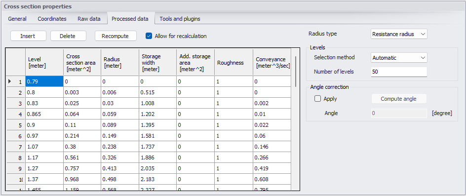
Figure: The Processed Data tab page on the Cross Section Properties panel

Details on these variables are given below:

Level: Levels for which processed data are calculated in the cross section. Default level definitions range from the lowest z-value and up to the highest z-value in the raw data table.
Cross section area: Effective cross sectional flow area calculated from the raw data. Effective area is determined from the total flow area adjusted by eventual relative resistance values different from 1 in the raw data tab.
Radius: Resistance or hydraulic radius depending on the selected type in the ‘Radius type’ dropdown list.
Storage width: Width of the water surface for the given water level.
Add. storage area: Additional storage area defined manually as a function of the water level. The purpose of the additional storage area is to include an additional volume of storage in the cross section, which is not represented by the geometry in the raw data. The calculated water level in this additional storage remains strictly the same as in the cross section. This is useful for representing small storages associated with the main branch such as a lakes, bays and small inlets. The additional storage area values describe the area of the water surface for a given water level. Additional storage areas are always user-defined; they will never be given a value from the automatic processing of the raw data.
Roughness: This factor can be used to apply a level dependent, variable roughness in the cross section. The roughness factor can contain the following two types of values depending on the Roughness Type definition in the raw data tab:
- Roughness type defined as relative roughness factor: In this case, the roughness value is interpreted as a factor by which the roughness numbers defined in the 'Bed roughness' editor will be multiplied or divided during the calculation in order to establish a level-dependent roughness in the section. That is, the roughness factor works as a level dependent roughness scaling factor in the current section.
- It is important to note in the case of relative roughness type that a factor higher than 1 will increase the actual roughness of the river bed, whereas a factor lower than 1 will decrease the actual roughness. So when the roughness type is Manning (M), then the Manning's M value is divided by this factor. When the roughness type is Manning (n), then the Manning's n value is multiplied by this factor.
- Roughness type defined as absolute roughness number (Manning’s n, Manning’s M or Chezy number): In this case, the roughness column contains the actual roughness number applied in the simulation. The roughness column can therefore have values of either Manning’s M, Manning’s n or Chezy numbers.
Conveyance: Conveyance values are not used in the simulation but is primarily displayed as part of the processed data for the purposes of checking that the conveyance is monotonously increasing with increasing water level, which is one of the key assumptions for open water hydraulics.

During the simulation, the processed data will be interpolated in order to cover the full range of water levels encountered during the simulation.

Tip

Processed data are essential in simulations as they describe the hydraulic properties for cross sections. Hence, it is important to inspect processed data and make sure that they accurately describe these hydraulic parameters. It is for example important to make sure that their plots are smooth in order to correctly reproduce progressive changes with changing water levels. If the plots show abrupt changes, it may be necessary to edit the levels at which processed data are computed. Additionally, a situation where the conveyance column is not monotonically increasing with water levels can occur, especially in the case of some closed sections or in situations where the section geometry includes a sudden width increase and the radius type has been set to ‘Hydraulic radius’. Should this occur, it is strongly recommended (not to say a strict requirement) to adjust the section characteristics such that a monotonically increasing conveyance curve is obtained. If not, there is a high risk of encountering instabilities in the simulation for water levels in the range where conveyance values are not monotonically increasing.

Typical options for optimising cross section characteristics for open sections is to use ‘Resistance radius’ types instead. Alternatively, when using the ‘Hydraulic radius’ type option, manually subdivide the section into several ‘slices’ by adjusting the relative roughness numbers in the raw data at locations where the section’s shape significantly changes (e.g. changing a relative roughness value from 1.000 to 1.001 ‘forces’ the processed data calculator to divide the integration of the processed data into several slices and the non-monotonically increasing conveyance curve can normally be resolved from this.

Note

The conveyance values presented in the conveyance column are actually not the ‘True’ conveyance values. Depending on the choice of roughness type in the ‘Processed data’ tab, the ‘True’ conveyance may depend on the roughness values specified in the ‘Bed roughness’ editor. However it has been decided to present conveyance values which do not consider these roughness numbers. Consequently, the conveyance shown in the processed data page does not reflect the true conveyance, but is primarily offered as a way for analysing the ‘conveyance trend’ as a function of water levels in the cross sections. These should be monotonically increasing with water levels to ensure healthy output from the simulations.

Insert and Delete Buttons¶

The ‘Insert’ button above the table can be used to insert a new line in the table, while the ‘Delete‘ button can be used to delete the active line.

Allow for Recalculation¶

Processed data values may be automatically recomputed when this option is checked. Values are recomputed when changes are made to cross section properties, when the ‘Recompute’ button in the tab page is pressed, or when the ‘Recompute all’ or ‘Recompute selected’ buttons in the ‘General’ tab are pressed. In case the processed data have been manually adjusted, one may need to uncheck this option to ensure manual adjustments are unchanged.

Info

Processed data are also recomputed when the setup is saved if ‘Allow for recalculation’ is active.

Recompute¶

This button is only active when the option ‘Allow for recalculation’ is checked. Pressing this button recomputes all the processed data in the table.

Radius Type¶

The radius type may be set as:

Resistance radius: A resistance radius formulation is used.
Effective area, hydraulic radius: A hydraulic radius formulation where the area is adjusted to the effective area according to the relative roughness variation.
Total area, hydraulic radius: A hydraulic radius formulation where the total area is equal to the physical cross sectional area.

Levels¶

Options for dividing the cross section into levels for processed data computation are:

Automatic: The levels are selected automatically. In case Radius Type is ‘Resistance radius,’ levels are selected according to variations in section flow width. For ‘Total area, hydraulic radius’ radius type, levels are selected according to variation in the section conveyance.
Equidistant: The levels are selected with equidistant level difference determined from the ‘Number of levels’ specified.
User-defined: The levels can be fully or partially user-defined. Define levels in the ‘Levels for processed data’ table accessed via the ‘Edit levels button. If the number of defined levels is less than required by the Number of Levels specification the remaining levels will be selected automatically.

Set the desired number of processed data levels via the ‘Number of levels’ parameter. The automatic level selection method may not use the full number of levels specified. This will occur when a smaller number of levels is sufficient to describe the variation of cross sectional parameters.

The ‘Edit levels’ button is only available if the level selection method is user-defined. The required levels are entered manually or pasted into the ‘Levels for processed data’ table.

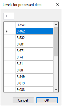
Figure: ‘Levels for processed data’ table

Angle Correction¶

An angle correction may optionally be applied to the cross section. The correction may be used for situations where the cross section profile is not perpendicular to the center line of the river. To activate the correction, the ‘Apply’ checkbox must be checked, and the angle must be manually specified.

The correction applied is simply a projection of the cross sectional profile on the normal to the thalweg of the river:

(3.2)

where q is as shown in the figure below.

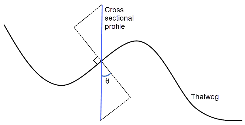
Figure: Correction angle for cross sections

Note

The correction of X-coordinates is not reflected in a change of S values in the raw data table, but only in the processed data table.

Cross Section Plot¶

The Cross Section Plot panel shows various data:

A single black line for the current cross section. The curve represents the values defined in the raw data table with the X axis describing the S values and the Y axis describing Z values plus the datum value.
Points shown with red circles on the plot indicate the locations of markers 1, 2 and 3. Points shown with blue circles represent markers 4 and 5
The blue curve describes the resistance values across the current cross section.
Optionally, a number of grey plots from different cross sections if the 'Draw history on plots' option in the 'General' tab is active.
Optionally, a green line describing elevations obtained from a selected DEM, if the option 'Draw DEM elevations', in the 'General' tab, is active.

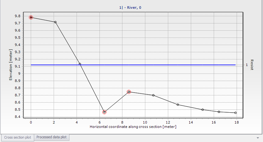
Figure: The Cross Section Plot panel on the Cross Sections editor

Note

To remove the history of cross section plots, right-click on the plot and choose ‘Clear history’ from the context menu.

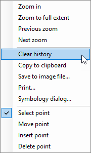
Figure: Context menu from the cross section plot

A number of options for the plot are available through the contextual menu. Right-click on the cross section plot to access the dialog (figure above).

The context menu includes the following three feature groups:

The first group of features relates to zooming facilities: Zoom in, zoom to full extent, and previous/next zoom facilities are available.
The second group of features relates to the appearance and export of the plot. From here you can export the image to the clipboard or to an image file on the disk, and you can also print it. Additionally, the symbology dialog allows changing the display settings of the plot.
The third group of features relates editing the active cross section's raw data on the plot. The following functions are available:
- Select: When active, it is possible to select a cross section point on the plot, which makes the point active in the raw data table. Pressing a number on the keyboard will assign the corresponding marker value to the selected point. Pressing the 'Ctrl' key + the number will remove the corresponding marker.
- Move points: When active, it is possible to move a point graphically on the plot. The raw data table will be updated accordingly.
- Insert: For adding new cross section points through the plot. Inserted points are interpolated between two existing points, and may be moved afterwards.
- Delete: For deleting points from the plot.

Processed Data Plot¶

The Processed Data Plot panel shows data for the current cross section, or also for a number of cross sections if the ‘Draw history on plots’ option in the ‘General’ tab is active.

The curve represents the values defined in the processed data table, with the Y axis describing the level values and the X axis describing one of the other items from the table (e.g. area, radius, width, additional storage, roughness, or conveyance). The plotted item is controlled by the dropdown list above the plot.

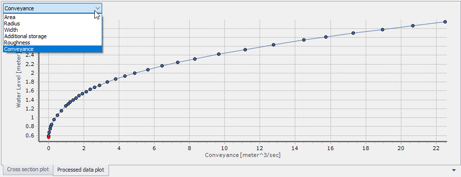
Figure: The Processed Data Plot panel on the Cross Sections editor

To control the settings and appearance of the plot, a number of options are available through a contextual menu. Open the menu dialog by right-clicking on the plot. Zooming and plot appearance options are offered on the context menu.