2D Fluid Properties
The hydrodynamic solver uses per default fluid properties describing clear water. It is however possible to simulate one-phase flows with different flow characteristics, e.g. oil or water with high concentrations of debris or mud. To enable this, select the 'Water loaded with mud or debris, or oil' type.
A flow resistance relationship for a flow regime equivalent to a Bingham or Non-Newtonian flow approach is calculated under the assumption that the debris-flow material behaves like a viscoplastic fluid. Fluids considered for this solution would typically be oil or debris flow with high concentrated mixtures of flowing sediments and water.
Fluid property parameters to be defined include: Fluid Density, Yield stress and Bingham fluid viscosity.
Note
2D Precipitation and evaporation, as well as 2D infiltration, are not available in connection with this alternative fluid type and the respective data pages are therefore automatically hidden when activating this option.
General Description
The 'Water loaded with mud or debris, or oil' type enables an alternative hydrodynamic solution in which a fluid dependent flow resistance is added to the standard flow momentum equations.
Naef et al (2006) defines a number of formulations for calculating flow resistance relations and the flow resistance term; \(t_{0}/r\). The current implementation includes a 'Full Bingham' relation, which in addition allows for applying simpler resistance formulations which excludes the Bingham viscosity term (e.g. the 'Turbulent and Yield' relation as defined in Naef et al (2006)).
The full Bingham flow resistance relation determine the flow resistance term (\(t_{0}/rgh\)) from the following third order equation (see Naef et al, 2006):
(3.1) 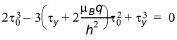
where q is the flux (discharge per unit width), h is the fluid depth, \(t_{y}\) is the yield stress and \(m_{B}\) is the Bingham fluid viscosity.
The third order equation is solved numerically during the simulation to give \(t_{0}\) as function of the yield stress (\(t_{y}\)), Bingham viscosity (\(t_{B}\)), water depth (h) and flux (q).
Note, that it is possible to activate e.g. the Turbulent and Yield resistance formulation by simply setting the Bingham Viscosity parameter, \(m_{B}\), equal to zero.
Recommended Values
The rheological properties of non-Newtonian fluid are driven by the complex interaction of a fluid's chemical and material composition. Key composition properties include the particle size distribution (e.g. percent fines), solids concentration, water content, chemical composition, and mineralogy such as the presence of clay minerals.
The Bingham rheological model is well suited for homogenous fluid mixtures with high concentrations of fine particles (e.g. mudflows, hyper-concentrations of fine sand, silt, and clay-size sediment) and other material types such as oils.
The key parameters for the Mud/Debris/Oil model are the following (default unit shown in brackets):
| Fluid density: | Density of the fluid mixture [\(\text{kg}/\text{m}^{3}\)] |
| Yield stress: | Shear stress threshold that needs to be exceeded for the fluid to flow [Pa] |
| Dynamic viscosity: | Dynamic viscosity of the Bingham fluid mixture [PS s] |
Fluid density
The fluid density can be determined from either measurements of the fluid to be modelled or calculated using the solids concentrations of the fluid mixture.
Yield stress
Ideally, the yield stress (i.e. yield strength) of the fluid to be modelled can be determined from rheograms developed from viscometric measurements in a laboratory. A rheogram relates the shear rate of the fluid to the applied shear stress. A commercially available concentric cylindrical viscometer is ideally suited for this type of analysis because it is capable of developing the rheogram for a wide shear rate range. However laboratory derived rheological analyses may not always be possible or practical.
Yield stress can also be determined empirically from both case studies involving similar fluid compositions and empirical relationships. For hyper-concentrations composed of fine sediment, yield stress is often formulated as a function of material type (e.g. clay mineralogy) and sediment concentration. Julien (2010) provides the following recommended empirical relationships for yield stress as a function of sediment concentration for a variety of material types using this exponential form:
(3.2) 
where \(t_{y}\) is the yield stress [Pa], a and b are coefficients (see table below) and \(C_{v}\) is the volumetric sediment concentration.
| Material | a | b |
|---|---|---|
| Bentonite (montmorillonite) | 0.002 | 100 |
| Sensitive clays | 0.3 | 10 |
| Kaolinite | 0.05 | 9 |
| Typical soils | 0.005 | 7.5 |
Table: Coefficients for yield stress empirical relationships from Julien (2010)
Oils are a special application where the yield stress is typically set to zero and the dynamic viscosity dictates the laminar flow nature represented by the Bingham rheological model. For zero yield stress the Bingham fluid model is valid for laminar depth-integrated flow.
Note
The typical exponential relationship between yield stress and sediment concentration indicates that at some point small changes in concentrations can dramatically change yield stress. This is an important dynamic sensitivity to consider when evaluating Bingham fluids.
Dynamic viscosity
Once the fluid is in motion, the dynamic viscosity (i.e. plastic viscosity) represents how the fluid flows under applied shear stresses. Similar to yield stress, the dynamic viscosity can be determined from rheograms developed from viscometric measurements in a laboratory. However laboratory derived rheological analyses may not always be possible or practical.
Dynamic viscosity can also be determined empirically from both case studies involving similar fluid compositions and empirical relationships. Julien (2010) provides the following recommended empirical relationships for yield stress as a function of sediment concentration for a variety of material types using this exponential form:
(3.3) 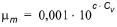
where \(m_{m}\) is the dynamic viscosity [Pa s], c is a coefficient (see table below) and \(C_{v}\) is the volumetric sediment concentration.
| Material | c |
|---|---|
| Bentonite (montmorillonite) | 100 |
| Sensitive clays | 10 |
| Kaolinite | 9 |
| Typical soils | 7.5 |
Table: Coefficients for dynamic viscosity empirical relationships from Julien (2010)
For modelling viscous, low-strength fluids such as oils, the dynamic viscosity is the key parameter for the Bingham model as the yield stress is often set to zero. The dynamic viscosity for such materials is best determined from rheograms developed from viscometric measurements in a laboratory, e.g. commercially available concentric cylindrical viscometer. Available literature (e.g. product descriptions) and case studies for commercially derived materials are other appropriate sources for choosing the value for the dynamic viscosity parameter.
Remarks and Hints
The Bingham fluid viscosity must be defined as a Dynamic viscosity.
When a Bingham formulation is activated and a resistance relation is calculated from this, the turbulent resistance (Bed resistance) defined by Manning or Chezy values should ideally be deactivated. However, in situations where Yield/Bingham stresses are not dominating, turbulent resistance may be crucial to maintain model stability, and hence, it is important to realize that turbulent resistance and the resistance relation from the Bingham solution are both active and included as individual resistance contributions in the hydrodynamic solution.