Theoretical Background¶

General description¶

MIKE+ Water Hammer simulates hydraulic transient (unsteady) flow in any fully pressurized pipe networks carrying liquids. MIKE+ Water Hammer provides a cost effective tool for engineers seeking fast answers to questions about rapid operation of piping systems. Water hammer is based on the high-order implicit scheme solving the continuity and momentum equation using the finite difference method. The initial conditions are modeled using MIKE+ standard water distribution module.

Water Hammer allows you to model:

Sudden changes in flows and pressures
Pump start-up and pump trip-off
Valve operations
Power or equipment failure events
Surge protection.

The water hammer computation is based on the Continuity equation:

(16.1)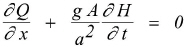

and the Momentum equation:

(16.2)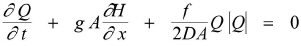

where:

Q is the discharge
H is the piezometric head above arbitrary datum
f is the Darcy-Weisbach friction factor
D is internal pipe diameter
A is the cross-sectional area of the pipe
g is the gravitational acceleration
a is the wave speed
x is the distance along the pipe axis
t is the time.

In the governing equations, the acceleration terms which are very small compared to the other terms have been disregarded.

Wave Speed¶

For pure liquids Halliwell (1963) presented the general expression for the wave speed

(16.3)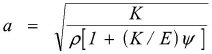

in which E is the Young's modulus of elasticity of the conduit walls, K is the bulk modulus of the fluid, r is the density of the fluid and y is a nondimensional parameter.

Rigid Conduit¶

(16.4)

Thick-Walled Elastic Conduit (D/e <= 10)¶

anchoring at both ends = full restraint:

(16.5)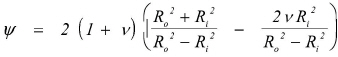

in which n is the Poison’s ratio, \(R_{o}\) is an external diameter, \(R_{i}\) is an internal diameter.

upstream anchoring = upper restraint:

(16.6)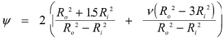

frequent expansion joints = expansion joints:

(16.7)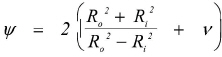

Thin-Walled Elastic Conduit (D/e > 10)¶

anchoring at both ends = full restraint:

(16.8)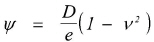

in which D is the conduit diameter and e is the wall thickness.

upstream anchoring = upper restraint:

(16.9)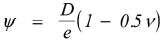

frequent expansion joints = expansion joints:

(16.10)

Tunnels Through Solid Rock, Parmakian 1963¶

Unlined tunnel:

(16.11)

where G is the modulus of rigidity of the rock.

Steel - lined tunnel:

(16.12)

in which e is the thickness of the steel liner and E is the modulus of elasticity of steel.

Reinforced Concrete Pipe¶

This pipe can be replaced by an equivalent steel pipe having equivalent thickness.

(16.13)

in which \(e_{c}\) is the thickness of the concrete pipe, \(A_{s}\) - the cross-sectional area of steel bars, \(L_{s}\) - the spacing of steel bars, \(E_{r}\) - the ratio of the modulus of elasticity of concrete to steel (0.06 - 0.1), but 0.05 for cracks.

Diagrams¶

The following diagrams can be used in order to estimate the wave speed.

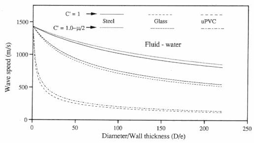
Figure: Relationship between wave speed and D/e for fluid water

Values of Young's Modulus of Elasticity and Poisson's Ratio for a range of common materials are available in the following table.

Material	Young's Modulus (\(10^{9} \, \text{N}/\text{m}^{2}\))	Poisson's Ration (-)
Aluminum	70	0.3
Cast Iron	80-110	0.25
Concrete	20-30	0.1-0.3
Copper	107-130	0.34
Glass	68	0.24
GRP	50	0.35
Polyethylene	3.1	-
PTFE Plastic	0.35	-
PVC Plastic	2.4-2.8	-
Reinforced Concrete	30-60	0.15
Rubber	0.7-7.0	0.46-0.49
Steel	200-24	0.3
Titanium	103.4	0.34

Table: Values of Young's Modulus of Elasticity and Poisson's Ratio for a range of common materials

Typical values of Bulk Modulus are:

\(K = 2.05 \times 10^{9} \, \text{N}/\text{m}^{2}\) for water
\(K = 1.62 \times 10^{9} \, \text{N}/\text{m}^{2}\) for oil.

Numerical scheme and algorithm¶

The numerical solution is based on the approach suggested by Verwey and Yu (1993). An implicit, space-compact finite difference scheme has been implemented for simulation in pipe networks including a variety of control elements. The same numerical scheme can be used for simulation of both hydraulic transients and water distribution problems. The inertia terms in the governing equations can be manipulated to produce relatively fast convergence for steady state problems.

The implicit finite difference formulation is based on a non-staggered grid in time and space, where at each grid point the independent variables Q and H are to be computed. The friction term in the governing equations has been expressed as

(16.14)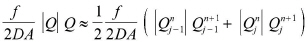

The coefficients for the water hammer model have been derived and have the following form:

(16.15)

(16.16)

(16.17)

(16.18)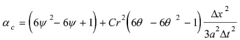

(16.19)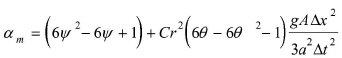

(16.20)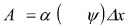

(16.21)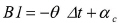

(16.22)

(16.23)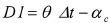

(16.24)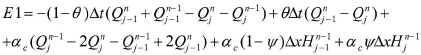

(16.25)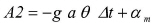

(16.26)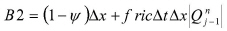

(16.27)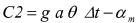

(16.28)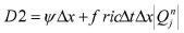

(16.29)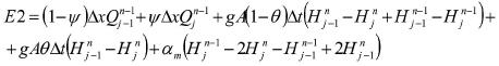

Looped network solution algorithm¶

The main algorithm generates a set of grid points using a finite difference scheme, see Cunge, Holly, Verwey (1980). The grid is introduced in time and space, where at every point the values of H and Q are defined as the unknown variables. Between the two successive grid points in time and space both the continuity and the momentum equation are applied. Together with the necessary boundary data, a sufficient number of equations are obtained to solve H and Q at every grid point.

The general form of the governing equations is

(16.30)

(16.31)

where coefficients A1, B1, C1, D1, E1 for the continuity equation and A2, B2, C2, D2, E2 for the momentum equation are derived from the high-order scheme.

The looped algorithm is based on the fact that a looped network contains elements known as nodes which represent the confluence of several flow paths, some of which originate from other nodes, some from boundary points. A system of simultaneous linear equations is developed where the piezometric head changes at each node are the only unknowns. Solution of this system by any matrix elimination technique yields the piezometric heads at each node.

Suppose that there are three links, 2-1, 2-3 and 2-4 and that there are b grid points along branch 2-3 and c grid points along a link 2-4, as shown in the figure below. For any computational grid point, the two equations below apply:

(16.32)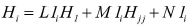

(16.33)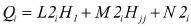

where L, M, N are functions of coefficients A, B, C, D, E, found through a double sweep elimination.

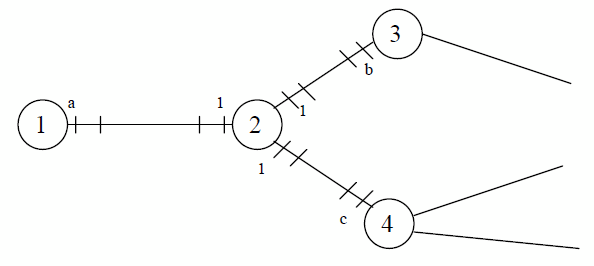
Figure: Part of a looped pipe network

These equations express the partial dependence of the unknown variables Q and H at any grid point in a branch on the value of H in the two adjacent nodes.

At internal nodes a compatibility condition must be satisfied. The simplest condition is node continuity and common piezometric head.

(16.34)

(16.35)

where n+1 indicates the (n+1)Dt time level in the solution, k is the index of the links emanating from node 2, and m is the number of such links. These relations can be written for each from M nodes, and this leads to a system of M linear equations having as unknowns the piezometric head changes H at each node.

(16.36)

where [S] is a coefficient's matrix, M x M elements, {h} is a vector of unknowns, M elements; {T(L)} is a vector of the free terms.

This system of linear equations may be solved by any matrix inversion techniques. Once the increments of piezometric head H are known at the nodes, it is possible to recompute Q(i) and H(i) values for all intermediate grid points through equations (16.34) and (16.35).

The looped algorithm may be described by the following steps:

The coefficients of the high-order scheme discretize the governing equations between two successive grid points on a branch.
The local elimination method is used to express Q and H grid point values on each branch in terms of H at the branch ends (nodes).
One equation for each node leads to the system of linear equations that is solved by the matrix elimination method.
Substitutions inside the branches yield the Q(i) and H(i) values for all intermediate grid points from the known values of H at the branch ends.

Hydraulic structures¶

The implementation of a hydraulic structure in the domain of the solution may be solved by replacement of the governing equations by another set of equations that characterise the particular hydraulic structure. Every time the main algorithm comes to the location of such a structure, it must switch between the governing equations. Any hydraulic structure can be implemented into such a numerical scheme in the following way. The hydraulic structure is placed between the two successive grid points, and we can assume that.

Another way of implementing a hydraulic structure is to handle it in the similar way to a node. The hydraulic structures are not located between the two successive grid points but in the node. Instead of modifying coefficients A,B,C,D, and E, we increase the number of linear equations.

The main algorithm is designed in such a way, that, after a process of linearisation and discretization of the governing equations, it solves them on a prescribed set of grid points using an appropriate numerical scheme. If a hydraulic structure is present in the domain of the solution, the algorithm must replace the governing equations by other equations defining a hydraulic structure in order to provide the numerical solution. Various hydraulic structures can be coupled together, e.g., the closing of one valve can determine the operating of another valve. In cases where this link exists between hydraulic structures, communication must be maintained and controlled by this main algorithm. This message has to be attached to the object in such a way that it represents the reality. Object-oriented design has been applied to create a safer interface to the numerical algorithm, since the low level operations that remain the same are hidden inside objects.