Water Hammer Simulations
Introduction
Water Hammer simulates transient (unsteady) flow in any fully pressurized pipe network carrying liquids. It provides a cost effective tool for engineers seeking fast answers to questions about rapid operation of piping systems.
Water Hammer allows you to model:
- Sudden changes in flows and pressures
- Pump start-up and pump trip-off
- Valve operations
- Power or equipment failure events
- Surge protection.
It handles any number of pipes, nodes, and loops in complex networks with various components.
Initial conditions are modeled using MIKE+ Water Distribution standard water distribution module. Additional settings used only for transient modeling are enabled when the model type is set to "Water hammer".
The following basic components are supported by the Water Hammer simulations.
| Component | Remark |
|---|---|
| Tank | Supported |
| Pump | Supported |
| Pressure reducing valve PRV | Not supported (*) |
| Pressure sustaining valve PSV | Not supported (*) |
| Pressure breaker valve PBV | Not supported (*) |
| Flow control valve FCV | Not supported (*) |
| Throttle control valve TCV | Supported |
| Closed pipes | Supported |
| Pipes with check valves CV | Supported |
| Node demands | Multiple junction demands including their patterns are kept constant during water hammer analysis. |
| Emitter | Supported |
Table: List of supported basic components
(*) replace the valve with a throttle control valve TCV and use the steady state valve opening (stroke position) as the initial valve opening in the valve operation schedule curve used in water hammer setup.
Several additional network components are used in Water Hammer simulations compared to EPANET-based simulation.
| Component | Remark |
|---|---|
| Air-chamber | Supported |
| Vented air-chamber | Supported |
| Air-valve | Supported |
Table: List of additional Water Hammer components
The following basic components are not supported by the Water Hammer simulations.
| Component | Remark |
|---|---|
| General purpose valve GPV | Not supported |
| Simple control rules | Not supported |
| Rule base controls | Not supported |
| Patterns | Demand and Reservoir patterns need to be entered as Transient Boundary Conditions |
Table: List of unsupported components
Running water hammer simulations
In order to be able to start water hammer simulations you have to prepare the steady state model and obtain satisfactory results. In the next step, you need to enable the Water Hammer analysis type in the 'Model type' editor, enter data used for transient analysis, define boundary conditions and computational parameters.
Initial conditions
Initial conditions are computed with the use of the steady state analysis. The results of the initial state are saved in the file as H, Q values at the beginning and end of the pipes respectively and in the vicinity of hydraulic structures such as valves, pumps, etc. There is a direct connection between the result file from initial conditions and the water hammer execution, in spite of the fact that the two models use different computational grids and different numerical engines.
Boundary conditions
There are in principle two types of boundary conditions, namely the piezometric head, H, above a specified datum, e.g., in tanks, and the discharge, Q, e.g., water demand. Both H and Q are given under selected names as time series in the Curve and Relations Editor and stored in the database. These boundary conditions may be assigned to any node in the network. Boundary for each time step is assigned from given time series specified by the user. If time step used by water hammer computation is smaller than appropriate neighbouring values in boundary conditions time series then linear interpolation is applied. There are nodes of the following types: H - boundary, Q - boundary, compatibility and structure (hydraulic component) description. It should be pointed out that time patterns, used in the Steady State Model, are ignored by the Water Hammer simulations.
For the Initial State for Water Hammer Model, the water level and/or discharges are constant in time. The boundary conditions using time series must be specified for a sufficiently long time interval.
Computational parameters
The most important numerical parameter is the time step. Since a numerical solution must be stable and as accurate as possible, you have to choose a proper value of \(D_{t}\). The stability condition is given by the Courant number
(16.37) 
in which a is the wave speed and Dx is the distance between two successive grid points. In principle, an implicit, space-compact scheme is unconditionally stable, with exact solutions generated for the Courant numbers Cr = 0.5 and Cr = 1.0, respectively. The scheme enables us to vary the Courant number over pipes while maintaining its high accuracy. Accurate results are produced in the range 0\< Cr \< 1.1. You should try to maintain the Courant numbers below unity, but as close as possible to Cr = 1.
The question how to choose the time step is dictated by the nature of the hydraulic transient itself and by the shortest pipes in the system. The time step can vary from the order of 0.001 to 10 seconds. The time steps must be small enough in order to describe very fast changes of variables. It is recommended to start with the shortest pipe section and to calculate the time step, considering Cr = 1. Pipe sections with high Courant numbers are numerically treated in MIKE+ Water Distribution as rigid pipelines. This simplification enables a user to deal with a very short pipe section which would not be important within the water hammer simulation.
Other general parameters can be controlled in the 'Water hammer' tab from the 'Simulation setup' editor, and are described below:
- Theta: Coefficient for offsetting the numerical scheme in time, the default is 0.5.
- Apha: Coefficient for offsetting the numerical scheme in space, the default is 1.
- Gravity acceleration: Gravitational acceleration, the default is 9.806 m/s\(^2\).
- Atmospheric pressure: Atmospheric pressure, also known as air pressure or barometric pressure, the default is 10.11 m.
- Vapor cavity pressure: Vapor pressure is the water pressure under which the water starts releasing air, the default is 0.25m.
- Temperature: This is the water temperature.
- Add unsteady flow friction: Unsteady flow friction is an addition to the standard "quasi steady" friction computation concept which is widely used in practice. Unsteady flow friction considers rapid flow acceleration and changes to the pipe flow direction under unsteady flow conditions. When this option is unselected, the total friction only considers quasi steady friction. When this option is selected, the total friction is the sum of quasi steady friction and unsteady flow friction.
Definition of network layout
An example of a topological representation of a network is shown in Fig.3.1. The solution domain consists of branches connected one to another by means of nodes. Grid points are generated along branches and they represent the place where we are looking for the solution of the governing equations. Different hydraulic structures can be included later at selected places in the network.
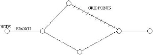
Figure: Definition Network Layout
For model construction, we can define a range of model elements such as nodes, branches, grid points and hydraulic structures.
Branches
Branches can be used to represent pipes of constant properties. In the pipe network, branches may include hydraulic elements, for example, valves, pumps. Nodes represent the applicable boundary conditions at the end of branches.
Nodes
Nodes are elements that represent free branch ends, branch connections or a specific storage. At nodes with one simple pipe connected, boundary conditions are usually defined by specifying the values of piezometric head or discharge as a constant value or as a function of time. Flow continuity and a piezometric level compatibility is assumed at nodes connecting several branches together.
Generally, there are these three different types of nodal boundary conditions:
- H (pressure (m) is given).
- Q (discharge (l/s) is given).
- Compatibility (common H).
Other types of nodes can be given as:
| Node Type | Meaning | Variable |
|---|---|---|
| H-Boundary | Given HGL | H=f(t) |
| Q-Boundary | Given Demand (inflow/outflow) | Q=f(t) |
| Continuity | Continuity | None |
| Junction node without demand | Continuity | None |
| Junction node with demand | Given Demand | Q=const |
| Tank | Calculated HGL | H=f(t), H=const |
| Air-chamber | Calculated HGL | H=f(t) |
| Vented air-chamber | Calculated HGL | H=f(t) |
| Air-valve | Calculated HGL | H=f(t) |
| Emitter | Calculated (pressure dependent) Demand | Q=f(t) |
Table: Node boundary conditions
Shaded VARIABLE types are set automatically by the program.
Grid points
Grid points are generated automatically by Water Hammer along the branches and they represent the computational grid where the values of piezometric head and discharge are solved and the input and/or output data are required. The program generates grid points based on the hydraulic time step entered by the user, wave speed given for every pipe and Courant number criterion. The system requires a different computational grid for steady state and water hammer computations.
Computational grid and hydraulics structures
The hydraulic components are located either in nodes or on branches. An example of grid-generation in a water distribution application with a valve illustrates the procedure of implementation of the hydraulic components. For water hammer applications the grid is defined as a function of the length of the pipe elements, the wave speed of water hammer and the speed of system operation.
Specific pipe data
Input of pipes is the same as in the case of steady state analysis. Then you have to specify the wave speed. Wave speed (celerity of the pressure wave) is the only one specific (and mandatory) parameter for the water hammer calculations:
- Wave speed: the sonic velocity is also the speed at which the pressure waves generated by water hammer travel in the pip (m/s or ft/s)
In case of a pipe with a check valve, the following fields need to be defined:
- check valve time to open: time interval to open the valve from closed position (sec)
- check valve time to close: time interval to close the valve from open position (sec)
- check valve cracking pressure: pressure that is required to open the valve (m or psi)
- check valve minimum velocity: velocity that is required to keep the valve open (m/s or ft/s)
- check valve is regulating: initial position of the valve i.e. if the valve is initially in the closed position (Yes/No)
- check valve idle interval: time interval that is needed before the valve close or open again (sec)
- check valve can reopen: setting that defines if the valve can re-open after it gets closed (Yes/No).
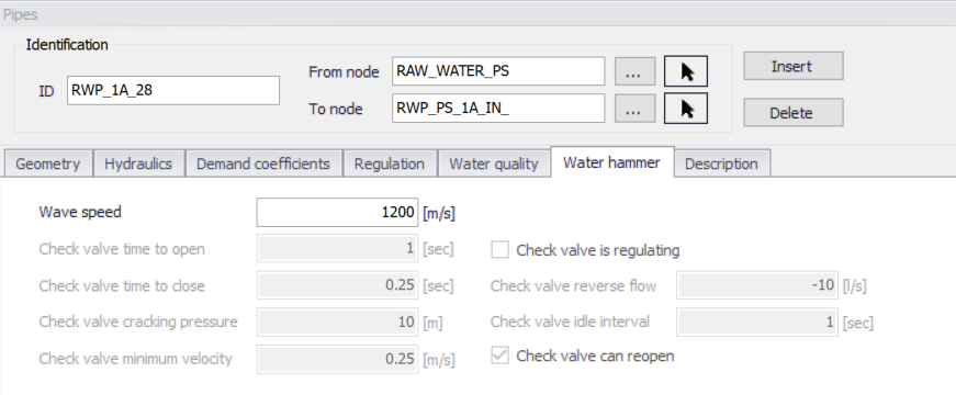
Figure: Pipe editor with water hammer settings
Junction node demands
Until specified as Water Hammer Boundary conditions, node demands are kept constant through out the water hammer simulation period. Junction demands i.e. multiple demands and their patterns - diurnal curves are use to calculate the steady state i.e. initial conditions for water hammer and they are kept on the same value for the water hammer analysis. Node elevation must be defined for every node.
Control rules
Simple Control Rules and Rule Based Controls are ignored during the water hammer analysis. Valve opening and pump scheduling is handled directly by the specific valve and pump data in Pumps and Valves editors and in Curves and Relations Editor.
Specific pump data
Input of pumps is the same as in the case of steady state analysis. Then you have to specify rated rotational pump speed and its schedule - time series of the rotational pump speed versus time.
Pumps may be located inside pipeline systems (booster pumps) or they may be connected to a suction well. Pumps are frequently used for various pipeline systems, and may operate during hydraulic transients with constant pump speed. Alternatively, the pump speed can decrease and/or increase depending on pump shut-down and/or pump start-up. The greatest difficulties come from hydraulic transient flows caused by turbopumps, since they may work in four quadrants. Four quadrants pumps are currently not supported.
There are in principle four dependent variables describing any state of a pump, namely:
- discharge - Q (m3/s)
- total dynamic head (tdh) - H (m)
- rotational speed - N (rpm)
- shaft torque - T (N.m).
The total dynamic head is defined as follows:
(16.38) 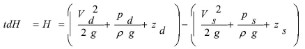
where the subscripts, d and s denote the discharge and suction flanges, respectively. Power input P (kW) is defined as:
(16.39) 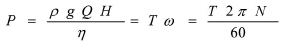
where h is the pump efficiency and T (N.m) is the torque which may be calculated from this equation.
Manufacturers may provide pump performance characteristics using other variables, e.g., {H, Q, N, P}, {H, Q, N, h}. If the pump operates only in the first quadrant, the typical pump characteristics {H, Q, N, h} for a given rotational speed of a centrifugal pump are shown in the figure below. The H - Q curve should be a monotonously decreasing function and then it is called a stable pump curve. The H - Q performance curve for a pump operating at constant rated speed may be approximated as:
H = b + aQ2
where b is the shut-off head and a is determined for maximum efficiency of the pump.
If the pump characteristics does not satisfy parabolic relation large errors may be produced in transient method and in all computation modules if the pump discharge is out of the Q-H curve.
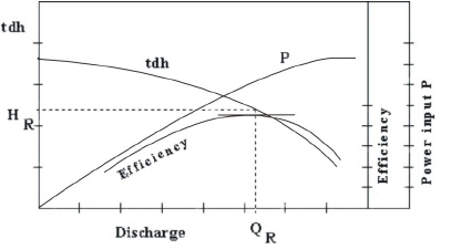
Figure: Pump Q-H Curve
Another performance characteristic curve which should be specified by the manufacturer is the net positive suction head (NPSH). The absolute pressure at the inlet flange of the pump should be above NPSH in order to avoid cavitation.
By applying the principles of dimensional analysis, the following relationships can be written for a pump operating at two different speeds N1, N2
(16.40) 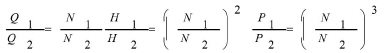
Subscripts 1 and 2 are only for corresponding points on an affinity law parabola. The affinity laws for discharge and head are accurate for all types of centrifugal pumps. However, large errors may be produced using the affinity law for a power requirement. It is recommended to compute P from head, discharge and efficiency and not from affinity laws.
Many of the important transient analyses situations are caused by start-up and shutdown of pumps. For a pump power failure the change in rotational speed of the pump depends upon the unbalanced torque applied
(16.41) 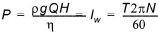
where \(I_{w}\) (N.m.s) is combined moment of inertia and \(D_{t}\) (s) is time step used for the calculation.
Pump start-up can be described by similar equation
(16.42) 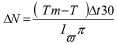
where, Tm (N.m) is the motor torque.
The relation between the pump speed and the total pump dynamic head is described by the following equation:
(16.43) 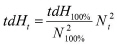
where, index (100%) represents the 100% of the pump rated speed and the time index t represents the actual value of tdH and N during the analysis.
Three different modes can be used in the transient flow analysis:
- pump is controlled by a pump operation schedule (N-time) curve
- pump is controlled by a pump operation schedule until time of the simulation is equal time of the power failure, then pump shutdown is applied and pump remains stopped till the end of the computation run.
- pump is primarily stopped (N equals zero) until time of pump start-up is reached, then pump start-up equation is applied.
Moment of Inertia, resistance of a rotating body to the change of its rotational speed, sometimes called rotational inertia. In linear motion, inertial mass is the measure of the resistance of a body to a change in its state of rest or uniform motion in a straight line. In rotational motion, moment of inertia is the measure of the resistance of a body to a change in its rate of rotation.The laws of motion of rotating objects are equivalent to the laws of motion for objects moving in a line, with moment of inertia replacing mass, angular acceleration replacing linear acceleration, and so on.
Force = mass x acceleration (F = ma) (linear motion)
Torque = moment of inertia x angular acceleration (T = Ia) (rotational motion)
The moment of inertia of a body can be calculated by dividing the object up into many small elements each with mass, m. If each element is a distance, ri, from the axis of rotation, the moment of inertia of the body is given by:
(16.44) 
The moment of inertia of a body depends on the axis about which the body is rotated. If two axes of rotation have different distributions of mass around them, then the body will have different moments of inertia for each of these axes.
Torque, a twisting effort applied to an object that tends to make the object turn about its axis of rotation. The magnitude of a torque is equal to the magnitude of the applied force multiplied by the distance between the object's axis of rotation and the point where the force is applied. In many ways, torque is the rotational analogue to force. Just as a force applied to an object tends to change the linear rate of motion of the object, a torque applied to an object tends to change the object's rate of rotational motion.
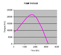
Figure: Pump torque curve
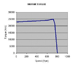
Figure: Motor torque curve
The following fields need to be entered in addition to water distribution modeling:
- Operation type:
- Pump schedule: pump operation is defined by a pump speed vs time curve
- Pump trip off: calculated pump trip off based on pump's data
- Pump start up: calculated pump start up based on pump's data
- Operation schedule: pump operation defined as pump speed vs time curve that is used before the pump starts up or fails.
- Rotational pump speed: pump speed (rpm)
- Moment of inertia: pump moment of inertia (\(\text{kg} \cdot \text{m}^{2}\) or \(\text{lb} \cdot \text{ft}^{2}\))
- Pump torque: pump torque (\(\text{Nm} = \text{m}^{2} \cdot \text{kg} \cdot \text{s}^{-2}\) or lb ft)
- Motor torque: motor torque (\(\text{Nm} = \text{m}^{2} \cdot \text{kg} \cdot \text{s}^{-2}\) or lb ft)
- Pump start up time: time when the pump starts up (sec)
- Pump trip off time: time when the pump trips off (sec)
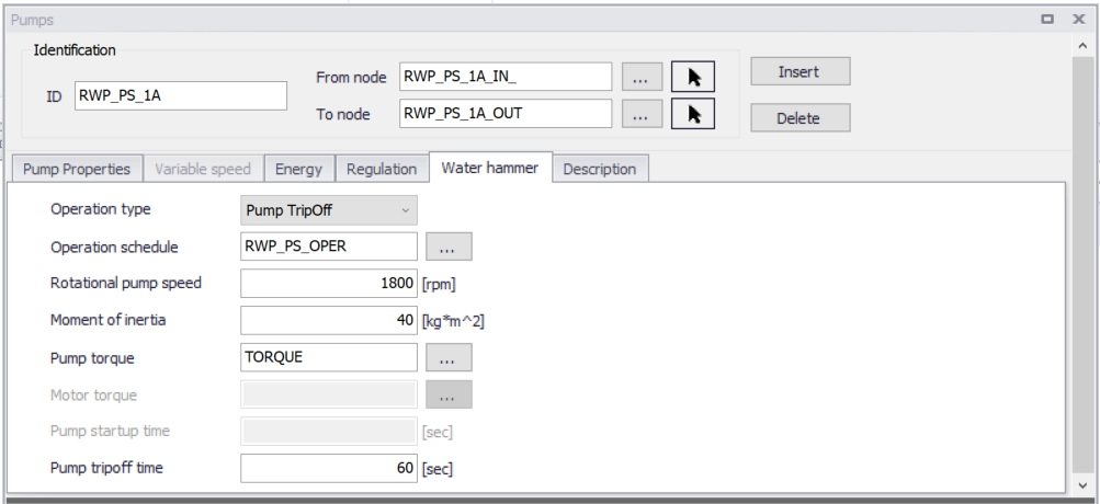
Figure: Pump editor with water hammer settings
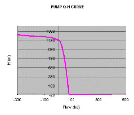
Figure: Pump Q-H curve defined for 100% rated speed
Specific valve data
Input of valves is the same as in the case of steady state analysis. Then you have to specify valve characteristic curve (in case of TCV valves) and valve schedule - relation between valve opening versus time.
The relationship between the flow Q and the head drop DH is expressed using a discharge coefficient Cd.
For an in-line valve, it reads:
(16.45) 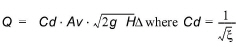
where Av is the valve area and x is the valve minor loss coefficient.
For a free-discharge valve, it reads:
(16.46) 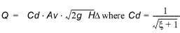
where x is the valve minor loss coefficient for a free-discharge valve.
Values of the discharge coefficients as functions of the relative valve opening (which is the ratio of valve and pipe area) have to be specified in the in Curve Editor. Typical representative data is of the following form
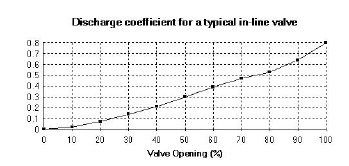
Figure: Discharge coefficient for a typical in-line valve
Note
TCV Throttle Control Valves can also be used as Isolation Valves for example for isolation of a pipe section in case of repair, isolation of a pump, etc.
The following fields need to be entered in addition to water distribution modeling:
- Operation schedule: valve opening (stroke position) vs time
- Valve characteristics: valve Cd or Kv coefficient vs time
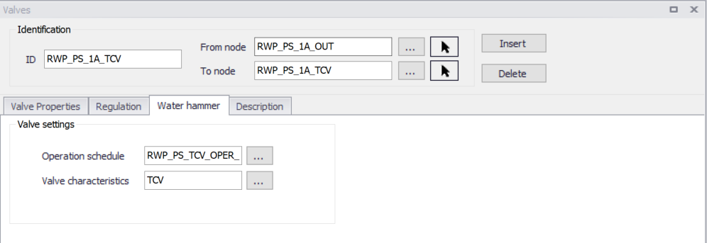
Figure: Valves editor with water hammer settings
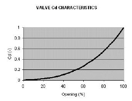
Figure: Example valve Cd Characteristics
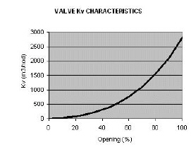
Figure: Example valve Kv Characteristics
The relation between Cd and Kv valve coefficients is given by the following equation:
(16.47) 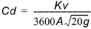
The relation between Cd valve coefficient and x minor loss coefficient is given by the following equation:
(16.48) 
or, for an in-line valve:
(16.49) 
Note
The valve minor loss coefficient used for the steady state analysis must correspond to the initial valve opening used for the water hammer analysis.
Specific project options settings
Currently, only SI units with LPS are allowed for the transient flow analysis along with Darcy-Weisbach friction expression, although results may be presented in custom units. Specific numeric parameters, such as theta (used to centre the high order finite difference scheme in time) and others can be defined.
Specific time settings
Running the fast transient analysis requires entering specific time setting, namely hydraulic time step and duration of the analysis. Pressure waves travels with a high speed in the pressurized pipe networks; wave speed in steel pipes is app. 1,200 m/s. In order to maintain Courant number criterion, dt - time step has to be very small number such as dt = 0.1s.
(16.50) 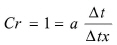
where: - a is the wave speed - dt is the time step - dx is the grid step - Cr is the Courant number.
Specific curves data
The following curve types below are available in the ‘Curves and relations’ editor, for use in Water Hammer simulations.
| Curve type | Description |
|---|---|
| HGL transient boundary | Define how HGL changes in time |
| Q transient boundary | Define how flow changes in time (positive value-outflow, negative value-inflow) |
| Valve schedule | Define valve opening and closing as a function of time |
| Valve characteristic | Flow coefficient versus valve opening |
| Pump schedule | Define pump starting and closing as a function of time |
| Pump torque | Pump torque versus flow |
| Motor torque | Motor torque versus pump rotational speed |
| Dual-acting valve characteristic | Air discharge versus gauge pressure |
Table: Curve data
Tanks
Surge Tanks have been widely used for hydroelectric systems in order to protect the low-pressure supply tunnel. They may also sometimes be suitable for water supply schemes. There are various types of Surge Tanks. The schematic presentation of common Surge Tanks is the same as mentioned above for Tanks.
The governing equations describing their hydraulic behavior are the dynamic equation and the continuity equation. Losses are disregarded at the junction, but are taken into account for pipes. Parameters characterizing the Surge Tank are:
Parameters:
- Node ID
- Maximum water depth above datum
- Starting water depth for computation
- Tank bottom level
- Tank Type:
- Rectangular tank: [a] [b] right prism rectangular tank, the base with sides a, b
- Circular tank: vertical cylinder with diameter D
- Variable: depth versus volume curve.
Air-chambers
Air-chambers contain compressed air which prevent very low minimum pressures in the pipeline and hence column separation. They are frequently used behind the pumps in water supply pipelines. Mostly they are cylindrical with a vertical and/or horizontal axis. A horizontal cylinder may be preferred for a very long pipeline when a large volume of air is required. The analysis is similar for both cases, but the computation of the volume of air in a horizontal cylinder is more difficult. The second figure below illustrates an air-chamber with a vertical cylindrical tank.
The hydraulic behavior of an Air Chamber is described by the relation between air pressure, its volume and continuity equation. It is assumed that the enclosed air follows the polytropic relation for a perfect gas
(16.51) 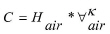
in which \(H_{air}\) and \(V_{air}\) are the absolute pressure head and the volume of the enclosed air, k is the exponent in the polytropic gas equation (k = 1.0 for an isothermal expansion, k = 1.4 for adiabatic expansion). The orifice losses are different for the inflow and outflow from the chamber.
The following fields need to be entered in addition to water distribution modeling:
- Polytropic expansion: the exponent in the polytropic gas equation (default value k=1.2).
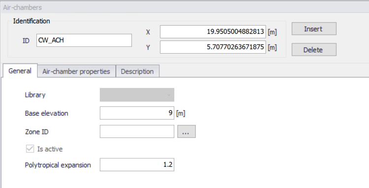
Figure: The Air-chambers editor with water hammer settings
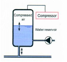
Figure: Air-chamber principle
Air-valves
Air-valves, similar to vented air-chambers, contain air which prevent very low minimum pressures in the pipeline and hence column separation. Air-valves are modelled as small vented air-chamber equipped by dual-acting valves that allow air to be sucked into its chamber and to escape therefrom, while preventing the outflow of liquid. When the pressure inside the surrounding pipes drops below the atmospheric pressure, air-valve opens and the air flow into a system. The proper valve characteristics are required to set by a user. As soon as the liquid starts flowing back into the dual-acting valve, valve closes.
The amount of air that is entering the air-valve during the sub-atmospheric conditions or leaving the air-valve during pressurized conditions is taken from the dual-acting valve characteristics. Next chart shows characteristics of Pont-a-Mousson, Ventex dual-acting valve, diameter of 150 mm.
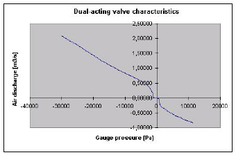
Figure: Dual-acting valve characteristics
When the pressure inside the air-valve drops below the atmospheric pressure, dual-acting valve opens and the air flows into a chamber. The proper valve characteristics must be defined by the user. As soon as the liquid starts flowing back out of the air-valve, the air-valve closes. The sizing of air-valve remains somewhat empirical, and it is recommended to contact the air-valve manufacturer as part of the design process.
The following fields need to be entered in addition to water distribution modeling:
- Valve diameter: diameter
- Polytropic expansion: the exponent in the polytropic gas equation (default value k=1.2).
- Dual acting valve curve: air valve characteristics.
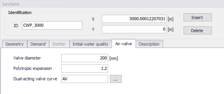
Figure: Air valve editor with water hammer settings
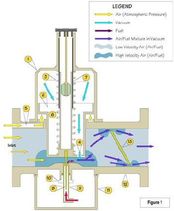
Figure: Air-valve principle