Error Forecast Equations

The correction relies on the difference between the observed value from the measurement time series and the simulated value. When observations are not available, this difference cannot be calculated, and the correction drops to zero. To avoid a sudden drop, a model for how the error should evolve during a period with no observations can be specified. The error forecast will be applied both after the last observed value (or after 'Time of forecast', whatever comes first) and during periods with missing observations (detected as delete values in the measurement time series).

The error forecast is a technique that relates to data assimilation using the 'Updating with weighting function' method, because a single-simulation method cannot preserve the error when the observation runs out of values (as ensemble methods can).

New equations are added or deleted using the 'Insert' or 'Delete' buttons at the top of the editor.

 

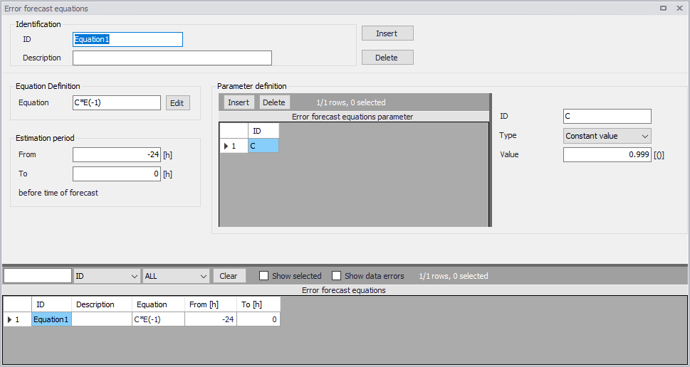
Figure: The Error forecast equations editor

Identification

ID: The identification name of the equation. This name will show up in the selection list for Error Forecast equations on the 'Weighting function' tab of the 'Update parameters' editor.

Description: An optional description of the equation.

Equation definition

Equations are specified in this 'Equation' field.

A special function available in the equation editor is E(L), which is the error computed at L time steps prior to the current time. The lag, L, must be prepended by a minus sign. A commonly used function is E(-1), which is the error at the previous time step.

The equation definition E(-1) will persist the last observed error throughout the forecast, so the last observed error will be added to the simulation result throughout the forecast.

A common model for fading out the error (instead of persisting it throughout the forecast) is to define an exponential decay. The equation for an exponential decay reads A*E(-1), where 0 < A < 1. The parameter A is the fraction of the error, which is maintained from one time step to the next, so the speed of the decay is determined by A. The larger A is, the more does the error in the current time step depend on the previous error, i.e. the slower is the decay. The half-life time of the error depends on A and on the time step of the model. Typically, one would be interested in calculating the A which results in a specific half-life time. The half-life time relates to A through:

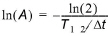
Where \(T_{1/2}\) is the half-life time and Dt is the time step.

Parameter definition

Parameters to be used in the Equation definition are specified here. Parameters are added or removed using the 'Insert' or 'Delete' buttons above the table.

ID: Identification name of the equation parameter. The name will appear in the 'Variables' list in the equation editor

Type: Equation parameters can be defined as one out of four types:

• Constant value: the parameter is assigned a constant value. If there are no plans to change it to an estimated parameter, the value might as well be written directly into the equation, e.g. 0.5*E(-1) is equivalent to A*E(-1) with A specified as a constant parameter with value 0.5.
• Estimated constant: a constant value with an automatic estimation performed to estimate the value from the computed time-varying error. Parameters that are specified to be estimated are not allowed as arguments to non-linear expressions (e.g. in the expression sin(a), a is not allowed to be estimated). The expression a*sin(x), where a is an estimated parameter (and x is not) is allowed.
• Time series: the parameter is assigned a time-varying value specified in an external time series.
• State variable: the parameter is a state variable, e.g. a computed water level or discharge at a grid point in the river network. One use of a state variable in an error equation could be to use an if-statement to distinguish between different flow situations, which can then have different error forecast models.

Depending on the selected type for the equation parameter, specific parameters must be defined. Specific parameters for 'Constant value' type include:

• Value: value assigned to the parameter.

Specific parameters for 'Estimated constant' type include:

• Minimum value: lower bound of the parameter.
• Maximum value: upper bound of the parameter.

Specific parameters for 'Timeseries' type include:

• File name: the path to the time series containing the values. The button to the right may be used to either browse, create or edit the time series.
• Item ID: this field shows the name of the item selected in the time series.

Specific parameters for 'State variable' type include:

• River ID: the river name where the state variable is located.
• Chainage: the chainage at which the state variable is located.
• Item: defines the type of state variable. Depending on the modules included in the simulation (in the 'Model type' editor), it can either be water level, discharge, or WQ component.
• WQ component: the name of the component from the Transport module, when the updated item is set to WQ component.

Estimation period

For parameters defined as 'Estimated value', automatic parameter estimation is applied based on the record of computed errors. The period of the record to be used for the parameter estimation must be specified relative to the time of forecast. The values in the 'From' and 'To' fields must be prepended by a minus sign. Positive values are not allowed as this would correspond to a time range in the forecast period. In most cases, the estimation period should cover the most recent "previous period", which is obtained by setting 'To' to zero.

This option allows the error forecast model to adapt from one forecast to the next, and thereby reflect the prevailing conditions at the time of forecast. For instance, the error forecast models can be adapted to the structural differences in the model errors that are often seen for different flow regimes.

Note

If the amount of observed data available before the time of forecast is not long enough to estimate the parameters in the error forecast equation, the updating location may be disabled. Be aware that estimating parameters on a long period will therefore increase the risk that the update is disabled, when only a limited set of observed data is available.