View Panels¶

MIKE+ includes four main panels by default to the left of the window:

Setup View: Tree structure with access to the data editors, where all data can be edited in forms or in tables. This tree view provides an overview of data validation to the model components by showing a green tick or a red cross next to each item. A red cross indicates that some records contain errors: open the corresponding editor to get more details on the error.
Layers and Symbols View: Lists the symbols and layers used in the Map. Allows you to configure graphics and model components symbols.
Results View: Lists all loaded result files in the project. Used for result presentation. The following buttons at the top are available to manage the files:
- Add file: this button allows to select new files to load in the project. While loading a result file, a window allows to select which result items from this file are to be loaded in memory, and which ones are to be shown as a layer on the map. Note that a result layer can be added to the map only if the corresponding result item is loaded in memory. If a result item is loaded but not added to the map at the same time, it can be added to the map at a later stage from the 'Layers and symbols' view.
- Add folder: this button inserts a folder to the tree structure to organize the list of result files.
- Remove: this button removes all the selected result files. Multiple files can be selected from the list using the Ctrl key, and selected files are highlighted in blue. An alternative option to remove all result files is available in the context menu (right-click on the list of files).
- Refresh: this button re-loads the result file.
- Properties: this button shows the result items from the result files which are currently loaded into the project, and allows to change the list of loaded items.
- Compare: this button compares two result files obtained from two different simulations but on the same network. Refer to Result Comparison for more information.
Plots View: Allows saving and organizing all types of result presentation windows, like time series plots, profile plots, results tables, result maps, etc. Refer to Plots Management for more information.

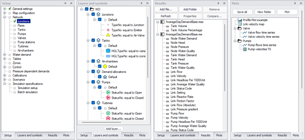
Figure: Setup, Layers and Symbols, and Results panels in MIKE+

A 'Property view' can also be shown, especially to display the properties of an item selected on the map with the 'Identify' button. It is by default opened on the right-end side of the screen. It can display properties from model data and from other layers added to the map, like elevation from a DEM at the selected location, attributes from a selected item from a feature layer, or result values. It contains a 'Layer' list at the top to control which layer to identify, using the following options:

Top-most layers: this option displays the properties of the item at the selected location from the first visible layer on the map, according to the order defined in the 'Layers and symbols' tree.
Visible model layers: this option displays properties only from the model data.
Or by selecting a specific additional layer (DEM, result file, or feature layer) from the list.

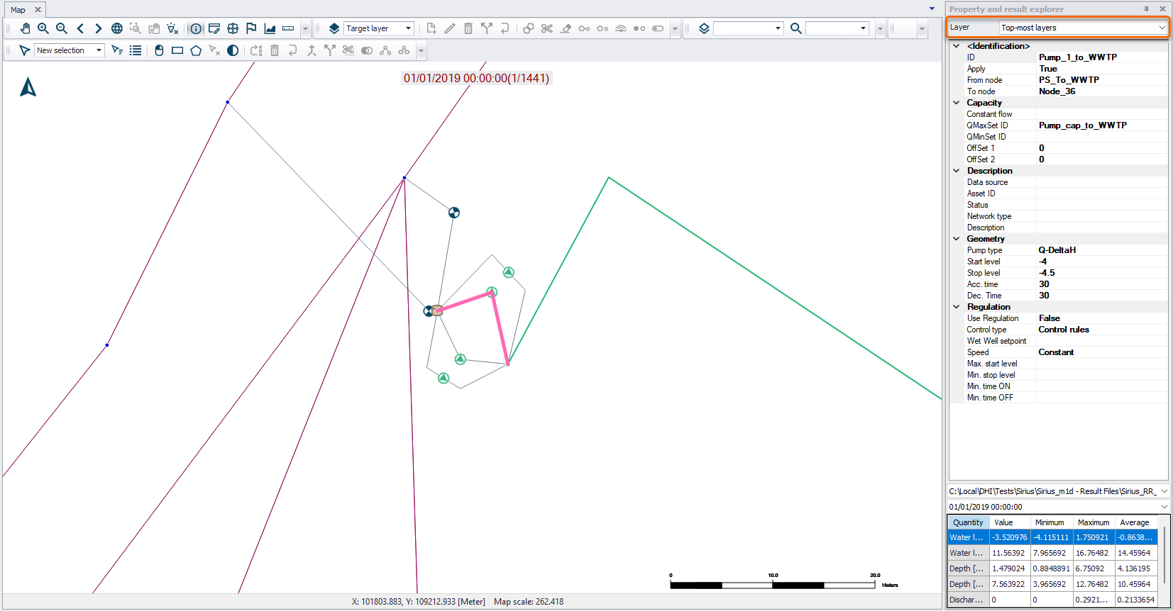
Figure: Controlling the source layer for the Identify tool

When displaying properties of the model layers, the Property view can be an alternative way to edit the data (instead of the main editor opened from the Setup view), which can easily be used side-by-side with the Map view. When 1D result files are loaded, this Property view also shows the results for the selected item.

When displaying properties of a layer from a .dfs2 file, the Property view shows additional J and K coordinates, which are the cell indices of the grid respectively along the horizontal and vertical axes. The cells numbering starts at 0, and the cell with coordinates J=0 and K=0 represents the lower left corner of the grid.

When selecting the option 'Visible model layers’, additional properties are available, depending on the selected button:

Properties: This shows the main information from the Property view, i.e. it shows the various data for the item picked on the map using the 'Identify' button, e.g. geometrical and hydraulic properties.
Default values: When this button is selected, the Property view shows the default values (used for future items to be created) for the item type which has been selected. For example, while editing nodes, this view will show the default values that will be applied when new nodes will later be created. These 'Default values' are common for all data in a given table, i.e. the values displayed in that mode are not specific to the selected item.
Status: When this button is selected, the Property view shows the attribute's status. Each attribute (property) for each record (item) can store a status information. This can e.g. be used to keep track of updates or to qualify the data.
Enum info: When this button is selected, the Property view shows the unit type (e.g. Water level) and the unit (e.g. [m]) used for each attribute in the edited table. This is especially useful if a different unit should be applied, in order to identify which unit type should be edited in the 'units customisation' dialog. These 'Enum info' are common for all data in a given table, i.e. the information displayed in that mode is not specific to the selected item.

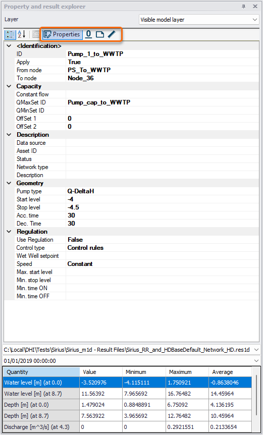
Figure: Model data in the Property view. Buttons in the rectangle control the displayed information

A 'Simulation view' can be used to display the various messages reported by the simulation engines while executing a simulation. This view is automatically opened when starting a new simulation.

A 'Log view' can be used to display various warnings and errors reported by MIKE+, for instance while using one of the predefined import and export routines, or when attempting to load invalid data on the map.

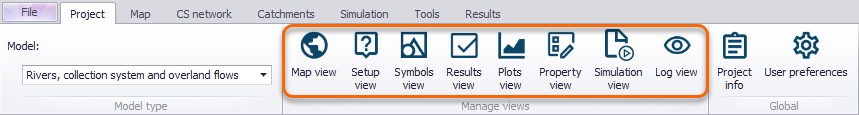
All these various Views can be opened via the ‘Manage Views’ toolbox on the Project tab in the ribbon, after they have been closed.

Working Modes¶

MIKE+ can operate in three different modes:

Rivers, collection system and overland flows
SWMM5 collection system and overland flows
Water Distribution

The working mode can be selected from the 'Project' tab in the ribbon, or from the 'Model type' menu in the Setup panel.

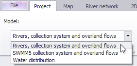
Choosing a specific working mode affects the visible layers on the Map view. However, regardless of the selected working mode, any layer contained in the database can be displayed by ticking appropriate group and layer check boxes in the Layers and Symbols View.

Alternatively, use the button 'View CS network' in the WD network tab in the ribbon, or the 'View WD network' in the CS network tab, which will also make the corresponding data layers visible on the map.

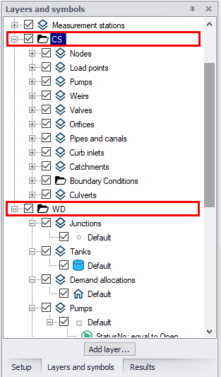
Figure: Working modes in the Layers and Symbols tree view

Map Layers¶

Various types of data layers can be shown on the Map view:

Background map: a background overlay, mainly from online sources, can be selected from the 'Background map' editor. Refer to the Background Map editor description for more information.
Model data layers: these layers show the model data, which are added in the various editors from the Setup View. The list of model data layers shown on the map is controlled by the working mode and the active features of the project, as defined in the 'Model type' editor.
Result layers: when a result file is available in the Results View, its results can also be shown on the map using dedicated layers. Result layers are by default added automatically on the map at the end of a simulation. They can also be manually added using the 'Add layer…' button in the Layers and Symbols View or in the Map tab of the ribbon.
External layers: additional layers from files containing GIS data can also be added to the Map view. They can be added using the 'Add layer…' button in the Layers and Symbols View or in the Map tab of the ribbon.

Info

Automatic addition of result layers at the end of simulations can be disabled from the User preferences dialog.

The following types of external layers can be added to the map:

Shape files (*.shp): a file containing either points, lines or polygons. Select the 'Feature layer' type in the 'Add layer' window, to select this type of file.
XYZ files (*.xyz): a text file containing scatter points, which can be used as input topography information for interpolating elevation on a 2D overland domain file. Select the 'Feature layer' type in the 'Add layer' window, to select this type of file.
CAD files (*.dwg, *.dxf): a file containing various types of drawings. Select the 'Feature layer' type in the 'Add layer' window, to select this type of file.
Geodatabase (*.gdb): a database containing feature layers. After selecting the database, the list of feature layers from the database to be displayed on the map needs to be selected. Select the 'Feature layer' type in the 'Add layer' window, to select this type of file.
BIM files (*.ifc): a Building Information Modelling file containing buildings drawings. After selecting the file, the list of feature layers from the file to be displayed on the map needs to be selected. A number of settings must also be specified to properly locate the file on the map: Coordinate system, Reference point location (identification of a reference point in the file), Reference point projected coordinates (location on the map of the identified reference point, expressed in the selected coordinate system), Rotation from true North (measured anticlockwise, from the reference point), Scale factor (e.g. used when the unit in the file is millimeters instead of meters). The specified settings are automatically saved to a *.xml file with the same name as the *.ifc file, and will be automatically reloaded the next time the *.ifc file is added to MIKE+. Select the 'Feature layer' type in the 'Add layer' window, to select this type of file.
dfs2 files (*.dfs2): DHI proprietary file format for raster files, containing e.g. input topography or results from a 2D overland model. Select the 'Raster layer' type in the 'Add layer' window, to select this type of file.
Raster text files (*.txt, *.asc): text file format for raster files, typically containing DEM data. Select the 'Raster layer' type in the 'Add layer' window, to select this type of file.
Arc/Info Binary Grid: file format typically containing DEM data. Select the 'Raster layer' type in the 'Add layer' window, to select this type of file.
TIFF files (*.tif, *.tiff): file format used for regular images or raster data (typically DEM data). To add a DEM or another type of raster file, select the 'Raster layer' type in the 'Add layer' window. Such raster layers must also store geographical coordinates information as metadata in the file (also referred to as GeoTIFF file). To add a regular image file, select the 'Image layer' type in the 'Add layer' window. Geographical coordinates from TIF images can either be read from the file's metadata (GeoTIFF file), defined manually or read from a world file (see World Files for Background Images page 124).
Mesh files (*.dfsu, *.mesh): DHI proprietary file format for flexible mesh files, containing input topography (*.mesh files) or results (*.dfsu files) from a 2D overland model. Select the 'Mesh layer' type in the 'Add layer' window, to select this type of file.
Bitmap files (*.bmp): image file. Select the 'Image layer' type in the 'Add layer' window, to select this type of file. Geographical coordinates from BMP images can either be defined manually or read from a world file (see World Files for Background Images).
JPEG files (*.jpg, *.jpeg): image file. Select the 'Image layer' type in the 'Add layer' window, to select this type of file. Geographical coordinates from JPEG images can either be defined manually or read from a world file (see World Files for Background Images).
PNG files (*.png): image file. Select the 'Image layer' type in the 'Add layer' window, to select this type of file. Geographical coordinates from PNG images can either be defined manually or read from a world file (see World Files for Background Images).

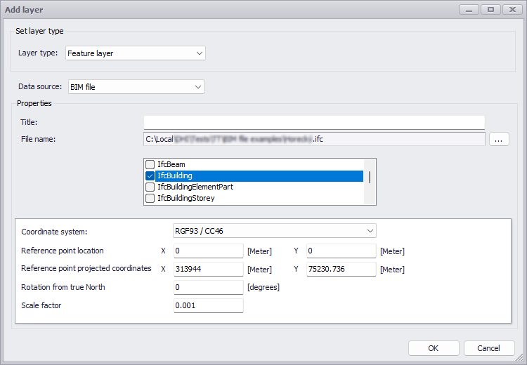
Figure: Providing settings to add a BIM file layer on the map

World Files for Background Images¶

Images may be added as background images for the Map in MIKE+.

Images are interpreted as raster data, where each cell in the image has a row and column number. In order to display images with GIS data, it is necessary to establish an image-to-world transformation that converts the image coordinates to real-world coordinates.

This transformation information is stored with the image.

Some image formats, such as GeoTIFF, and ESRI grids, store the georeferencing information in the header of the image file. MIKE+ uses this information if it is present.

However, other image formats store this information in a separate ASCII file. This file is generally referred to as the world file, since it contains the real-world transformation information used by the image. World files can be created with any editor.

World file naming conventions¶

It is easy to identify the world file which should accompany an image file: world files use the same name as the image, with a "w" appended. For example, the world file for the image file mytown.tif would be called mytown.tifw.

How georeferencing information is accessed¶

The image-to-world transformation is accessed each time an image is displayed (e.g., when you pan or zoom). The transformation is calculated from one of the following sources, listed in order of priority:

The world file
The header file (if the image type supports one)
From the row/column information of the image (an identity transformation)

Because a world file has higher priority, you can override the header file transformation information by creating your own world file.

World file contents¶

The contents of the world file will look something like this:

20.17541308822119
0.00000000000000
0.00000000000000
20.17541308822119
424178.11472601280548
4313415.90726399607956

When this file is present, MIKE+ performs the image-to-world transformation. The image-to-world transformation is a six-parameter affine transformation in the form of:

x1 = Ax + By + C
y1 = Dx + Ey + F

where:

x1 = calculated x-coordinate of the pixel on the map
y1 = calculated y-coordinate of the pixel on the map
x = column number of a pixel in the image
y = row number of a pixel in the image
A = x-scale; dimension of a pixel in map units in x direction
B, D = rotation terms
C, F = translation terms; x,y map coordinates of the center of the upper-left pixel
E = negative of y-scale; dimension of a pixel in map units in y direction

Note

The y-scale (E) is negative because the origins of an image and a geographic coordinate system are different. The origin of an image is located in the upper-left corner, whereas the origin of the map coordinate system is located in the lower-left corner. Row values in the image increase from the origin downward, while y-coordinate values in the map increase from the origin upward.

The transformation parameters are stored in the world file in this order:

20.17541308822119 - A
0.00000000000000 - D
0.00000000000000 - B
-20.17541308822119 - E
424178.11472601280548 - C
4313415.90726399607956 - F

Boundary Conditions Displayed on the Map¶

Boundary conditions are per default displayed on the Map. To be displayed, boundary conditions must be applied and contain at least one ‘Boundary Item’.

To ensure the Map view reflects all recent boundary condition changes, access the Map local context menu (i.e. right-click) and select the ‘Refresh boundary visualization’ option.

Collection System and River network¶

The different boundary conditions that can be visualized for collection system networks are seen in the figure below.

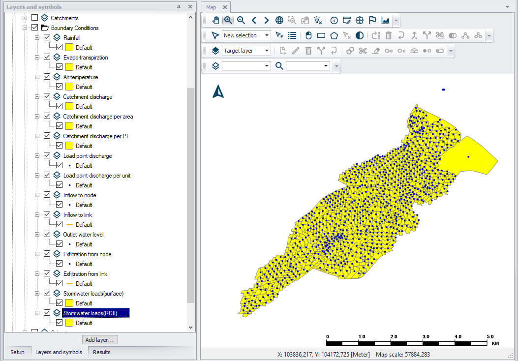
Figure: CS network boundaries

For further information on Collection System Boundary Conditions, please refer to the relevant chapter in the MIKE+ Collection System User Guide.

Similar boundary conditions for river networks can also be displayed on the map.

Water Distribution¶

Node demands can be displayed by ticking the Water Node Demands layer. Per default, the different demand categories will be differentiated when displayed.

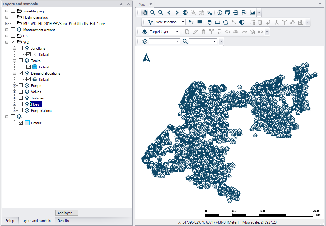
Figure: WD demand allocation points

Symbology settings¶

Labelling and symbology for layers on the main Map View may be customized via the Symbology Settings dialog.

On the Symbols and Layers panel, click on the symbol to edit (initially called "Default") under the desired layer. This will open the Symbology Settings editor shown below).

Set parameters inside the Symbology and Label tabs to customize the appearance of the layer on the main Map.

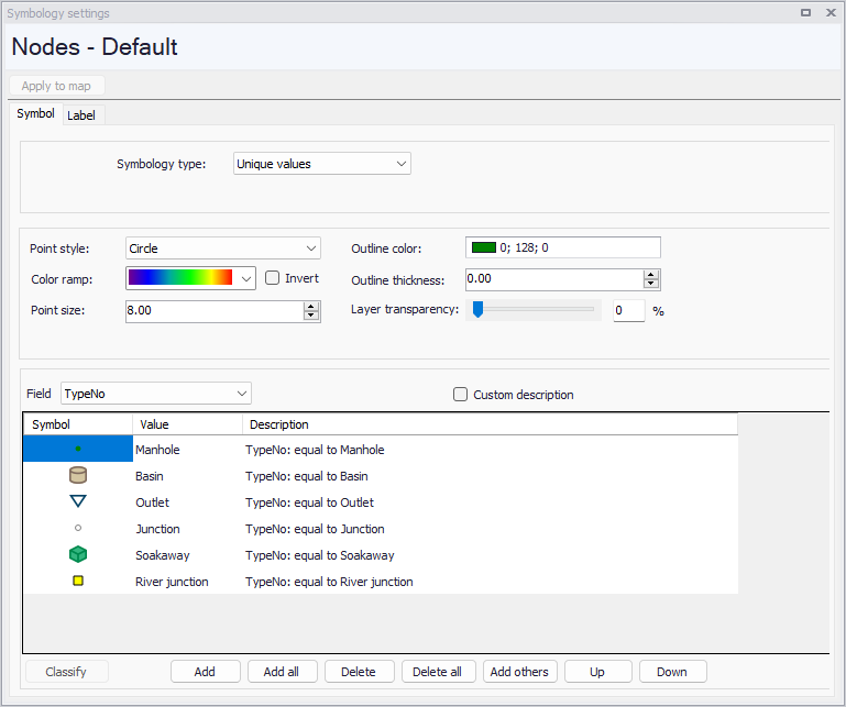
Figure: Symbology Settings dialog from the Symbols and Layers view panel

It is possible to configure multiple symbology settings for the same layer, to easily switch between them. To do so, right-click on a symbol (e.g. "Default") under the desired layer and select "Duplicate symbol". Right-click the different symbols to rename them as necessary. Then simply tick the symbol to apply on the map for the layer. Note that only the active symbol can be edited in the 'Symbology settings' editor.

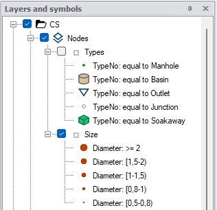
Figure: Defining multiple symbols for a layer

Custom symbol settings can be saved to a file for later re-use. Right-click on the symbol, the layer or the group of layers and select 'Save symbology' to save respectively a single symbol, all symbols for the selected layer or all symbols for all layers in the folder. Then right-click on a layer or a group of layers in another project to load the settings from the file.

Also see Labelling and Symbology to edit symbology settings from result maps.

Symbol¶

The Symbol tab holds settings to control the appearance of the selected layer on the map.

Available settings differ depending on the two categories of layers below:

Points / polylines / polygons features: this category covers the most common features in MIKE+ projects, displayed as points / polylines / polygons on the map (e.g. pipes, nodes, catchments, rivers, etc.), as well as external feature layers added to the map (e.g. shape files). For this type of layer, it is possible to control the symbol(s) representing the features as well as their size and color.
Raster and other 2D overland layers: this category covers external raster layers (e.g. DEM), input 2D overland files (e.g. 2D domain file) as well as 2D overland results. For this type of layer, it is possible to control the color palette representing values of the mapped item in the file, to show or hide isolines, and to show or hide cells / mesh elements.

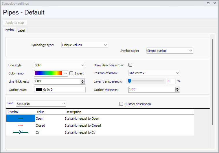
Figure: The Symbol tab showing settings for feature layers (left) and raster and 2D layers (right)

Settings available for feature layers are described in the following table.

Item	Description	Usage
Symbology type	Dropdown menu for selecting symbology type: - Single symbol - Graduated color - Graduated size - Unique values - Range values	Yes
Point style	Dropdown menu for selecting point symbol type	If point layer
Fill color	Color for point symbol	If point result layer and Symbology type = Graduated size
Symbols size from _ to _	Minimum and maximum range of symbol size to use	If Symbology type = Graduate size
Line style	Dropdown menu for selecting line symbol style	If line layer
Color ramp	Dropdown menu for selection of color ranges to use in symbolizing values	If Symbology type = Graduated color
Invert	Checkbox for inverting the application of the color ramp to the range of values	Yes
Point size	Point symbol size	If point layer
Line thickness	Line symbol thickness	If line layer
Outline color	Symbol outline color	Yes
Outline thickness	Symbol outline thickness	Yes
Draw direction arrow	Checkbox option for showing direction arrows. For pipes or rivers, this will show the direction of the link. For result layers, it can show the flow direction.	Yes
Position of arrow	Position of the arrow along the link geometry: - Mid vertex - End vertex	If Draw direction arrow = Active
Layer transparency	Slider for controlling the transparency of the layer on the map	Yes
Custom description	Checkbox for allowing customization of the symbology descriptions	Yes

Table: Feature layer settings in the Symbols tab

The dialog allows for changing symbol size, color, and value classes. E.g. one may wish to have links displayed by color, applying four different colors over the range of values.

Use the 'Classify' button in the dialog to define the number of classes to use and the break values for each class.

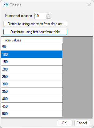
Figure: Customizing value classes for the symbology

In this classification window, the 'Distribute using min/max from data set' button will distribute equidistantly the specified number of classes using the minimum and maximum values of the feature layer being edited, for the field being classified. The 'Distribute using first/last from table' button will distribute equidistantly the specified number of classes using the first and last custom values specified in the table in this classification window.

Settings available for raster and 2D overland layers are described in the following table.

Item	Description	Usage
Auto-scale palette to visible data	Scales the defined color palette to match minimum and maximum values for current map extent, and also for current time step (for animated 2D results). When this option is active, the values of the color palette are recomputed when moving the map, when zooming in/out or when animating results. The number of values and the corresponding colors in the palette remain unchanged when the palette is recomputed. This may slow down the display when applied at large map scales and to large files.
Transparency	Percentage value controlling the transparency of the layer on the map.
'Palette' button	Button offering options to create a new palette, edit the current one, save the current one to a file, or load the palette from a file.
Shade type	This controls how values from the cells / elements are shown on the map. Three options are available: lNo contour: cells / elements are not colored. This may be used while displaying the cells / elements border instead, to keep another layer visible underneath. lBox contour: each cell / element is given a uniform color according to its value. This method is best for viewing actual data from the file. lShaded contour: this method provides smoothed contours between the different ranges of values from the color palette, using a bilinear interpolation of values from neighboring cells / elements. It is best for presentation purpose, but colors can locally deviate from the raw value in the cell / element, especially for results along edges of the flooded area.
Isoline visible	Option for displaying isolines between the different ranges of values from the color palette. Isolines are always smoothed using a bilinear interpolation of values from neighboring cells / elements.
Isoline label visible	Option for displaying isolines' values as labels along isolines.	Only available if isolines are displayed.
Remove adjacent identical labels	Option for removing neighboring labels along a common isoline.	Only available if isolines' labels are displayed.
Remove colliding labels	Option for removing overlapping labels.	Only available if isolines' labels are displayed.
Draw border	Option for displaying the borders of the grid or mesh with a black polyline.
Draw cells	Option for displaying the grid cells or mesh elements with a user-defined color and thickness.
Color	The color of the grid cells or mesh elements borders.	Only used when drawing cells.
Thickness	The thickness of the grid cells or mesh elements borders.	Only used when drawing cells.

Table: Raster and 2D layers settings in the Symbols tab

Label¶

To add labels to a map, tick the 'Visible' option in the 'Label' tab of the symbology editor. Multiple options are provided to control the position of the label, its font, number of decimals displayed and when to hide the label.

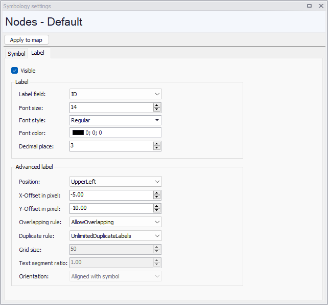
Figure: The Label tab

The following settings can be used to control the labels on the map:

Visible: Check box for showing or hiding the labels on the map
Label field: Parameter's values to display in the labels. For a result layer, the only available fields are the ID and the time series value. The 'Custom expression' option allows to define an expression combining multiple fields (not available for river cross sections).
Expression: this holds the expression of the label, when the label field is defined with the 'Custom expression' option. It is recommended to edit the expression in the Expression Editor. Such expressions can be displayed on multiple lines on the map, either by pressing 'Enter' in the expression editor or by using the NewLine function.
Font size
Font style
Font color
Decimal place: The maximum number of digits displayed after the decimal separator. This is only used when the labelled field is a numerical value, and does not apply when the numerical value is combined into a custom expression (in custom expressions, use the Round function instead).
Halo color: The color of the outline of the label.
Halo size: The size of the outline of the label. Set the size to 0, should no halo be used.
Position: A list of predefined locations of the labels, relative to the location of the corresponding features on the map. It is only available for point features.
X-Offset in pixel: Offset of the labels along the X-axis, relative to the specified 'Position'. A positive value will move the labels on the right, and a negative value on the left.
Y-Offset in pixel: Offset of the labels along the Y-axis, relative to the specified 'Position'. A positive value will move the labels downward, and a negative value upward.
Overlapping rule: Controls whether overlapping labels are allowed or not.
Min. labels spacing: When overlapping labels are allowed, this controls the number of overlapping labels displayed. The smaller the minimum spacing, the more overlapping labels.
Duplicate rule: This controls whether duplicate (identical) labels should be displayed, and how. This is not relevant when labels display e.g. IDs which are unique, but may be relevant to display uniform properties like material, zone ID, etc. There are three options to handle duplicate labels:
- No duplicate labels: this will remove all duplicates, i.e. only one label will be kept.
- One duplicate label per quadrant: this will remove duplicate labels only if they are in the same quarter of the screen. The screen will be divided into four quadrants, and when two duplicate labels are in different quadrants, they will both be kept.
- Unlimited duplicate labels: this will keep all duplicates.
Text segment ratio: This allows removing labels where the label length would greatly exceed the line length. It is a maximum ratio between the label length and the line length, above which the label is not shown. For example, when the ratio is set to 1, then the label will be suppressed if it is longer than the line. If the ratio is lower, then the label will be shown only if it is shorter than the line. If higher, then the label may be shown even if it is longer than the line.
Orientation: For line layers, the labels are by default aligned with (i.e. parallel to) the feature line on the map. This option can be used to force all labels to be horizontal.

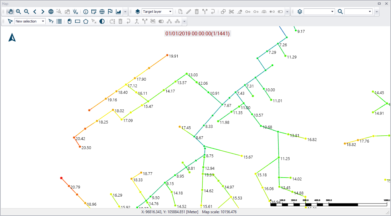
Figure: Example label configuration showing max.water level at nodes

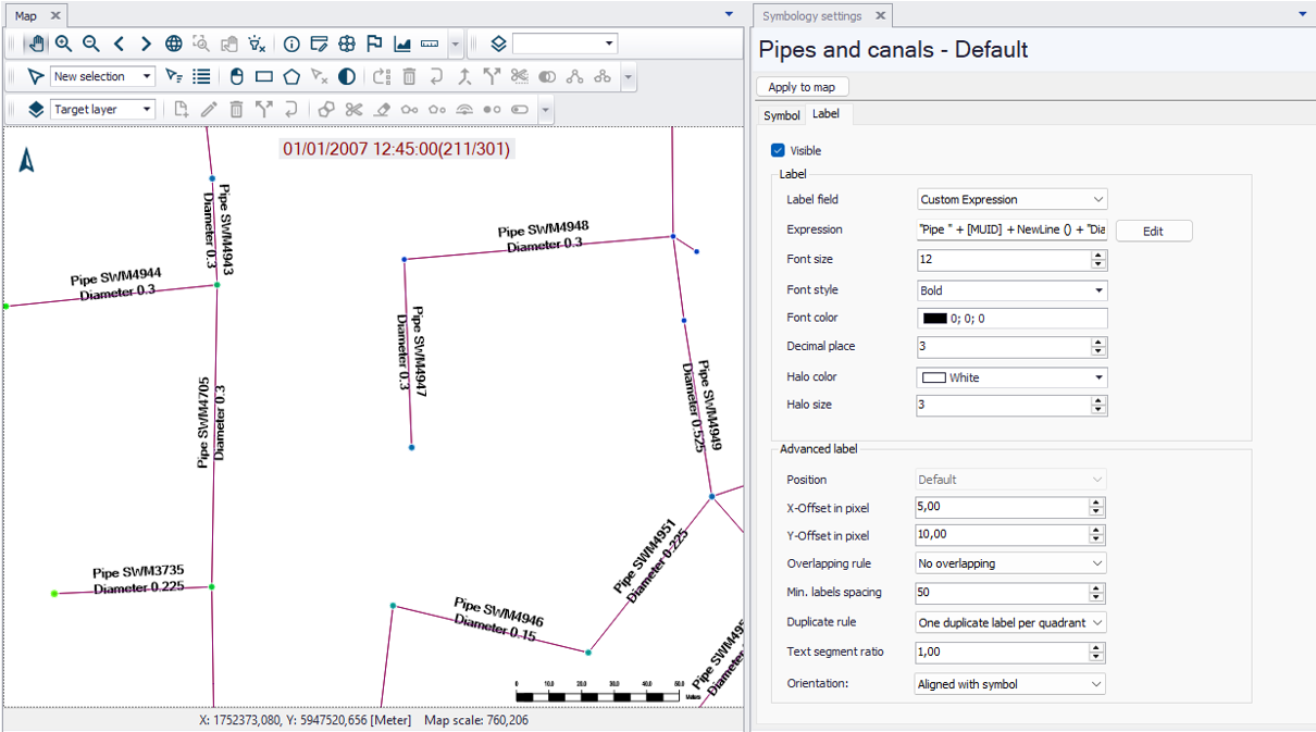
Figure: Example label configuration showing pipe ID and diameter using a custom expression

Also see Labelling and Symbology to edit symbology settings from result maps.