2D WQ Boundary Conditions

MIKE+ 2D Overland offers options for simulating transport of materials (e.g. pollutants) via the ‘Transport (AD, SWQ)’ module.

At present, 2D WQ computations are not available for models of type ‘SWMM5 collection system and overland flows’, and so options for defining 2D WQ boundary conditions are not offered for these types of models.

Options for setting-up 2D WQ boundary conditions are made available when both the ‘Hydrodynamic (HD)’ and ‘Transport (AD, SWQ)’ 2D Overland modules are activated for models of type ‘River, collection system and overland flows.’

 

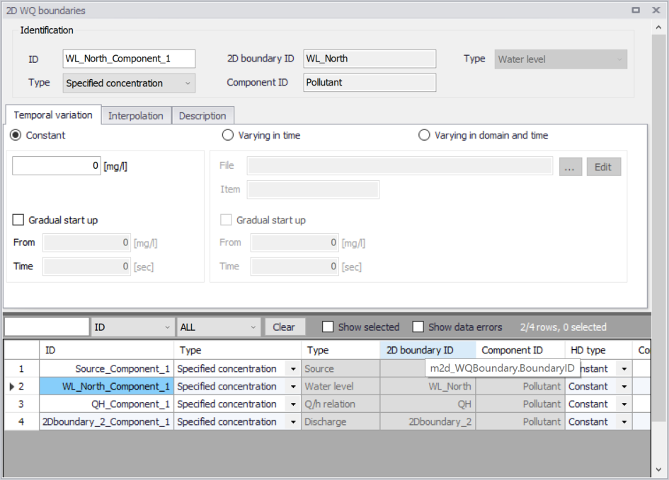
Figure: The 2D WQ Boundaries editor is automatically filled when water quality components have been defined in the model with open 2D boundary conditions that have been set up

Water quality AD (Advection-Dispersion) computations are based on flow conditions from hydrodynamic calculations. As such, water quality boundary conditions are specified in association with (i.e. attached to) open 2D hydrodynamic boundary conditions.

That is, hydrodynamic boundary conditions must first be set-up, after which water quality conditions are attached to them. Also, water quality components to be simulated must be pre-defined in the model through the WQ Components editor.

The main steps involved in defining 2D WQ Boundary Conditions are:

1. Define water quality components to be simulated in the WQ Components editor.
2. Set-up hydrodynamic boundary conditions in the 2D Boundary Conditions editor. See Chapter 2D Boundary Conditions for details on setting up hydrodynamic boundary conditions.
3. Access the 2D WQ Boundaries editor, and configure the automatically-detected open HD boundaries for associated water quality characteristics. Details on the various parameters for configuring 2D WQ boundary conditions are described in succeeding sections.

Identification

 

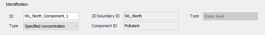
Figure: The Identification group box on the 2D WQ Boundaries editor

This group box contains general information on each 2D WQ boundary condition shown in the overview table at the bottom of the editor:

• ID: Unique ID for the 2D WQ boundary condition. The default ID is ‘2DBoundaryID_ComponentID’, where 2DBoundaryID and ComponentID are the IDs for the 2D boundary condition and the WQ component related to the active row from the overview table, respectively.
• Type (WQ boundary): 2D WQ boundary types vary depending on the associated HD boundary. More details on 2D WQ boundary types are found in the succeeding section.
• 2D boundary ID: The ID for the related 2D boundary condition. It is non-editable.
• Component ID: The unique ID for the related WQ component. It is non-editable.
• Type (HD boundary): The type of related 2D HD boundary condition (e.g. Discharge, Water level, etc.). It is program- detected and non-editable.

Possible 2D WQ boundary types vary depending on the associated HD boundary.

Source boundaries

Point sources of dissolved components are important in many applications such as release of nutrients from rivers, and intakes and outlets from cooling water or desalination plants. Associated water quality properties for Source boundaries may be defined as:

• Specified concentration: With this definition, the source concentration is the specified concentration if the magnitude of the source is positive (i.e. water is discharged into the ambient water). Otherwise, the source concentration is the concentration at the source point if the magnitude of the source is negative (i.e. water is discharged out of the ambient water). This option is pertinent to e.g. river outlets or other sources where the concentration is independent of the surrounding water.
• Excess concentration: For this option, the source concentration is the sum of the specified excess concentration and concentration at a point in the model if the magnitude of the source is positive (i.e. water is discharged into the ambient water). The source concentration is the concentration at the source point if the magnitude of the source is negative (i.e. water is discharged out of the ambient water). This type can be used to describe e.g. a heat exchange or other processes where the temperature (heat) or salinity is added to the water by a diffusion process.

The source flux is calculated as the product 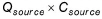, where \(Q_{source}\) is the magnitude of the source and \(C_{source}\) is the component concentration of the source.

Other bounday types

For most HD boundary types (i.e. Discharge, Water Level, Q/h Relation, and Free Outflow), WQ boundaries may be:

• Specified concentration: With this definition, the boundary concentration is the specified concentration for inflows into the domain (i.e. water is discharged into the domain). Otherwise, the boundary concentration is the concentration at the boundary if water is discharging out of the domain.
• Zero normal gradient: For this option, the concentration at the boundary is assumed to be identical to the concentration at the adjacent interior cell/element.

Temporal Variation

Temporal variation options are offered via the Temporal Variation tab on the 2D WQ Boundaries editor. Temporal variation is relevant only for concentration type WQ boundaries (i.e. 'Specified concentration' type).

The parameters offered on the tab vary according to the 2D (HD) boundary type associated with the WQ boundary, as indicated in the 'Identification' group box.

 

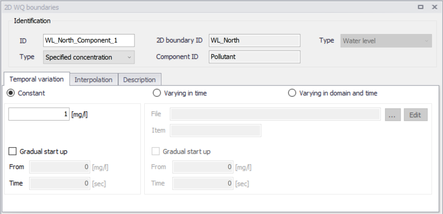
Figure: The Temporal Variation tab page on the 2D WQ Boundaries editor

Source Boundaries

Temporal variation options for Source water quality boundaries differ slightly from those for other types.

 

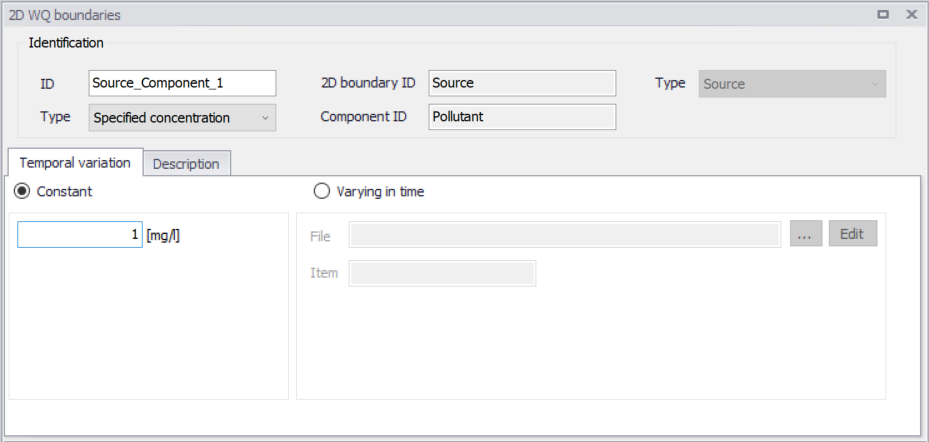
Figure: Temporal variation options for 2D Source water quality boundary conditions

Source WQ boundaries may be:

• Constant
• Varying in time: This option requires a timeseries (*.DFS0) data file containing concentration values (in concentration units) for the source. The data must cover the complete simulation period, but the time step of the input data file does not have to be the same as the time step of the computation. A linear interpolation of timeseries concentration values is applied if the time steps differ.

Note

Point sources are entered into elements in a way that the inflowing mass of the component is initially distributed over the element where the source is located. Therefore, concentration simulation results are usually lower than the specified source concentration.

Other boundary types

For most types of related HD boundaries (i.e. Discharge, Water Level, Q/h Relation, and Free Outflow), the temporal variation of ‘Specified concentration’ type WQ boundaries may be:

• Constant (in time and along boundary)
• Varying in time (and uniform along boundary): Requires a *.DFS0 data file containing the component concentration (in component unit) in the setup.
  • The data must cover the whole simulation period, although the data time step does not have to be the same as the simulation time step. This may require value interpolation during computations, for which an interpolation method may be specified on the Interpolation tab (See Interpolation).
• Varying in domain and time: This option requires a *.DFS1 data file containing information on component concentration (in component unit). and spatial variation.
  • The data must cover the complete simulation period, but the time step of the input data file does not have to match he simulation time step. This may require value interpolation during computations, for which an interpolation method may be specified on the Interpolation tab (See Interpolation).
  • In addition, spatial mapping of the *.DFS1 data file values to the boundary section must be specified on the Interpolation tab page.

You can specify a soft start interval during which boundary values are increased from a specified reference value to the specified boundary value in order to avoid shock waves being generated in the model. The increase follows a linear variation. To use this option, tick on the ‘Gradual start up' check box on the tab page:

• From: The component reference value for the soft start. The unit of the component is shown on the right.
• Time: The desired soft start duration.

Interpolation

Interpolation options are offered for 2D WQ boundaries expressed as concentrations (i.e. ‘Specified concentration’ type) except for 'Source' 2D boundaries.

Time- and space-wise interpolation settings may be defined in the Interpolation tab page of the 2D WQ Boundaries editor.

 

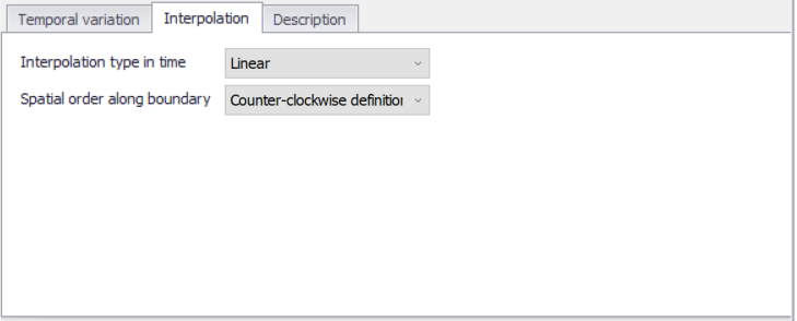
Figure: The Interpolation tab on the 2D WQ Boundaries editor

The 'Interpolation' tab offers options for the following:

• Interpolation type in time: For time-varying boundary types, the time step of the related timeseries (*.DFS0) file does not need to match the hydrodynamic calculation time step. Thus, value interpolation may be required during computations. Time-wise interpolation options are:
  • Linear: Values obtained from a linear function (straight line) between 2 known value points.
  • Piecewise cubic: Values obtained from a cubic polynomial approximation over sub-intervals.
• Spatial order along boundary: In cases where values vary along the boundary (e.g. Varying in domain and time), two methods of mapping the input data file (i.e. *.DFS1) to the boundary section are available:
  • Counter-clockwise definition: The first and last points of the line (i.e. *.DFS1) are mapped to the first and the last nodes along the boundary section, respectively, and the intermediate boundary values are found by linear interpolation.
  • Clockwise definition: The last and first points of the line are mapped to the first and the last nodes along the boundary section, respectively, and the intermediate boundary values are found by linear interpolation.

Description

Annotations for each 2D WQ boundary item may be added in the Description tab.

 

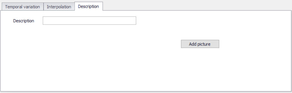
Figure: The Description tab in the 2D WQ Boundaries editor