Boundary Conditions Editor¶

Catchment boundary conditions¶

The list of available boundary condition types depends on the type of features included in the model setup (catchments, collection system network and/or river network). Types of variables associated with catchment boundary conditions are:

Air temperature
Evapotranspiration
Rainfall
Catchment discharge
Stormwater loads
Groundwater abstraction
Solar radiation
Degree-day coefficient
Catchment irrigation

Any number of each boundary conditions types can be specified.

Air Temperature is a boundary condition used for snow melt calculations and describing constant or time series varying temperature. This type of boundary is used for RDI hydrological calculations.

Evapotranspiration is a boundary condition describing potential evapotranspiration. This type of boundary is used for RDI hydrological calculations.The dfs0 file needs to be of the type ‘Evapotranspiration’. Delete values will be considered equal to 0.0.

Rainfall catchment boundary condition can be defined using a constant value, a uniform time series (from .dfs0 file) or using a spatially- and time-varying file (.dfs2 file). The latter format can only be used when the spatial extent of the boundary is set to 'Grid distributed weights'. This type of boundary is used for precipitation-runoff hydrological calculations. When using a time series the dfs0- or .dfs2 file needs to use one of the following Item Types: ‘Rainfall Intensity’, ‘Rainfall’ or ‘Rainfall Depth’. Delete values will be considered equal to 0.0.

Catchment discharge is a boundary condition of the type ’catchment load’, has associated to a discharge (constant, cyclic or a time series). This type of boundary represents various kinds of hydraulic loads, such as area-based or PE-based dry weather loads, area-based infiltration, etc. The discharge can be associated with any pollutant, sediment or temperature item (constant, cyclic or a time series).

Stormwater loads are boundary conditions only used when the Transport module is also included in the simulation. For this boundary type, the stormwater flow value is obtained from the hydrological model and cannot be specified in the 'Boundary conditions' editor: the purpose of this boundary type is only to associate the stormwater flow to a pollutant or sediment concentrations from the 'WQ boundary properties' editor. Select the boundary type 'Stormwater loads (RDI)' for catchments modelled with the RDI hydrological model. Select the boundary type 'Stormwater loads (surface)' for catchments modelled with any of the other hydrological models. For the boundary type 'Stormwater loads (RDI)', a flow type must also be selected (Total runoff, Overland flow, Base flow, etc.), to specify to which flow component of the RDI model the pollutant or sediment concentration should be associated.

Groundwater abstraction is a boundary type used with the RDI hydrological model, when the 'Use abstraction' option is active in the RDI parameters and when the pumped depth is defined as varying in time. The item type defined in the selected time series must be 'Ground Water Abstraction Depth'.

Solar radiation is a boundary type used with the RDI hydrological model, when snowmelt modelling is included and when the 'Use solar radiation' option is active. The item type defined in the selected time series must be 'Sun radiation'.

Degree-day coefficient is a boundary type used with the RDI hydrological model, when snowmelt modelling is included and when the 'Degree-day coefficient type' is defined as varying in time. The item type defined in the selected time series must be 'Melting coefficient'.

Catchment irrigation is a boundary type used with the RDI hydrological model, when the 'Include irrigation' option is active in the RDI parameters. The item type defined in the selected time series must be 'Irrigation'.

As the first action after inserting a new boundary conditions, a proper name (ID) must be specified. It is recommended to use a descriptive ID.

In order to include a boundary condition in a simulation, the 'Apply' box must be checked.

The selected type of boundary condition controls which options are active in the different tabs.

The following chapters describes the workflow to define a boundary condition for a catchment.

Network boundary conditions¶

In MIKE+ there is a single boundary condition editor for all types of network boundary conditions. The list of available boundary condition types depends on the type of features included in the model setup (catchments, collection system network and/or river network).

The following types of boundary conditions are available for collection system and/or river networks:

Load point discharge: this boundary condition is linked to a load point, and the inflow is specified in the 'Load points' editor
Load point discharge per PE: this boundary condition is linked to a load point, and the inflow and the number of person equivalents are specified in the 'Load points' editor
Inflow to node: a discharge boundary condition applied to a node from the collection system network
Inflow to link: a discharge boundary condition applied to a link from the collection system network
Inflow from result file: a discharge boundary condition where the discharge time series are obtained from a result file from a previous simulation. This is usually a .res1d file containing Rainfall-Runoff results or Catchment discharge results. It can alternatively be a .dfs0 time series file, or a SWMM result file (regular .out file or outflow interface file in .txt format). The boundary condition's spatial extent is automatically defined by the actual content of the selected result file and by the catchment connections defined in the MIKE+ project, therefore it is not possible to choose individual time series from the selected file.
Outlet water level: a water level boundary condition applied at an outlet of a collection system network. Only one water level boundary condition is allowed at each network outlet. If no boundary condition is specified for an outlet on a collection system network, a free outflow is assumed.
Exfiltration from node: an exfiltration boundary condition applied to a node from the collection system network. . It is defined as an infiltration rate. For a manhole, the infiltration area considered during the simulation is the circular area of the manhole, and for a basin it is the surface area of the water surface, which varies in time.
Exfiltration from link: an exfiltration boundary condition applied to a link from the collection system network, expressed as a flow per unit of length along the network.
Open inflow to river: a discharge boundary condition applied at the end of a river
Source inflow to river: a discharge boundary condition applied along a river. It can either be a point source applied at a point location, or a distributed source where the specified discharge is distributed evenly between a start point and an end point.
River water level: a water level boundary condition applied at the end of a river
River Q/h relation: the boundary condition at the end of a river is defined by a Q/h relationship, controlling the water level at the boundary as a function of the outflow.
Free river outflow: When the free outflow type is applied, the smallest of the critical and the natural depth is applied at the boundary
Closed river boundary: the closed boundary type is used at river end points where a zero-flux condition across the boundary is applicable.
Inflow to storage: a discharge boundary condition applied to a storage node from the river network.
Network rainfall: rainfall boundary conditions are specified in river reaches or storages where the inflow of rainfall on the channel is to be represented. The rain intensity applies to the water surface, i.e. the wet part of the river or storage area (hence excluding dry areas of the cross sections). Rainfall can be specified globally (spatial extent = All, applying to all rivers and storages), as a distributed source on selected rivers, or on selected storages. When applied globally, the network rainfall boundary condition can be defined using a constant value, a uniform time series (from .dfs0 file) or using a spatially- and time-varying file (.dfs2 file). When applied locally, it can only be defined using a constant value or a uniform time series (from dfs0 file).
Network evaporation: evaporation boundary conditions are specified in river reaches or storages where loss of water from evaporation from the channel is to be represented. Evaporation can be specified globally (spatial extent = All, applying to all rivers and storages), as a distributed source on selected rivers, or on selected storages. When applied globally, the network evaporation boundary condition can be defined using a constant value, a uniform time series (from .dfs0 file) or using a spatially- and time-varying file (.dfs2 file). When applied locally, it can only be defined using a constant value or a uniform time series (from dfs0 file).
Wind friction: wind friction on the water surface is accounted for by including wind shear stress in the simulation. When wind friction is applied, at least one wind friction boundary condition must apply to the entire network (spatial extent = All), to define a default wind field. Extra local wind boundary conditions may be added with local values and will take priority over the global wind field. When a wind friction boundary condition is included, a related 'Wind scaling factors' editor appears in the tree view, to specify local scale factors.
Groundwater leakage: the groundwater leakage boundary condition represents an additional loss of water from the river to the groundwater. When the groundwater leakage boundary condition is included, a related 'Leakage coefficients' editor appears in the tree view, to specify the coefficients (global and local coefficients) controlling the rate of the leakage. The groundwater leakage boundary condition can be defined using a constant value, a uniform time series (from .dfs0 file) or using a spatially- and time-varying file (.dfs2 file).

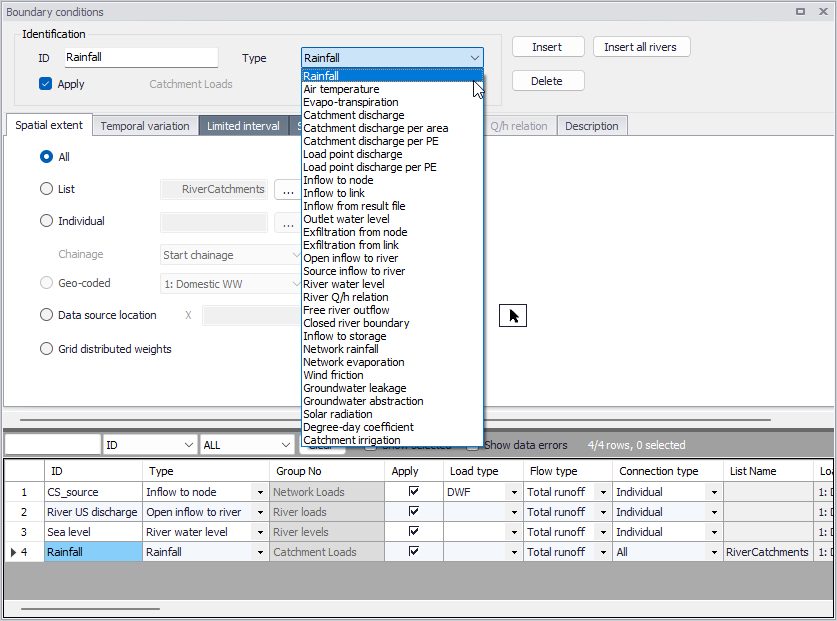
Figure: Hydraulic Boundary Conditions dialog

In order to include a boundary condition in a simulation, the 'Apply' box must be checked.

The selected type of boundary condition controls which options are active in the different tabs.

Defining HD Boundary conditions¶

Below are steps for defining basic HD boundary conditions in MIKE+.

Insert a boundary condition using the 'Insert' button on the upper right part of the Boundary Conditions editor. It is recommended to specify a descriptive ID for the new boundary condition.
Define the boundary condition type via the 'Type' dropdown list. The selected type influences subsequent data requirements for the boundary condition presented in the various tabs in the editor.
Define the location or spatial extent for the boundary condition in the Spatial Extent tab.
Define the values for the boundary condition item in the Temporal Variation tab of the editor.
Ensure the 'Apply boundary' checkbox is ticked if the boundary condition shall be used in subsequent simulations.

Special options and data requirements vary according to the boundary condition type defined, and so additional parameters/steps may be needed for other specific boundary types.

The subsequent sections describe the various options available in the various tabs of the Boundary Conditions editor in greater detail.

!!! note For river networks, boundary conditions are mandatory at river ends not connected to other parts of the modelled network. Rather than inserting and locating these boundary conditions manually, clicking the "Insert all rivers" button will add all the open boundaries of the river network to the boundaries table simultaneously. The created boundary conditions will be correctly located at the open ends, with a pre-defined boundary type: you then need to review the applied type, and specify the temporal variation of each boundary condition. If a boundary condition has already been defined at an open end, it will be kept unchanged when using the button.

Spatial extent¶

The 'Spatial extent' tab enables the modeller to define the distribution of the boundary conditions. The distribution ranges from 'All' (e.g. all catchments or all rivers, depending on the boundary condition type), Individual (specified locations), ‘List’ of a selection of elements (pipes, nodes, rivers or catchment depending on the boundary condition type), ‘Geo-coded’ locations, ‘Data source location’ and “Grid distributed weights”.

The application of ‘All can be applied to applied to catchment boundaries (‘Catchment discharge’, ‘Catchment discharge per area’ and ‘Catchment discharge per PE’). It can also be used for meteorological boundaries applied to catchments (‘Rainfall’, ‘Air Temperature’ and ‘Evapotranspiration’) or to the network (‘Network rainfall’, ‘Network evaporation’, and ‘Wind friction’).

Lists can be used with various types of boundary conditions to assign the condition to multiple items at once. Lists apply for a set of e.g. catchments, rivers, nodes or links, contained in a defined selection. The selection must first be saved in the Selection Manager, and then selected in the boundary condition definition.

'Individual' applies for a single item (catchment, river, node or pipe), and requires a specification of the item ID.

'Geo-coded' option applies to ‘Load point discharge’ and ‘Load point discharge per PE’ and is used to assignr Load points (typically DWF) geo-coded to the network nodes. User can select which one of the geo-coded load categories applies for this boundary condition.

Further information regarding the Geo-coding of loads is discussed specifically under the ‘Load Points’ help section.

'Data source location' allows assigning the XY coordinates of a rainfall gauge to the measured time series. With this option, each catchment will be assigned the closest rainfall time series. If one rainfall boundary condition is defined by 'Data source location', then all other catchment rainfall boundary conditions must also be defined with the same location type.

‘Grid distributed weights’ can be used to assign spatially varying rainfall data. The application of 2D radar data as input for runoff computations requires that rainfall dagta are defined in DHI’s dfs2 format files. MIKE 1D will automatically distribute the rainfall to individual catchments and apply it to the runoff computation.

Note

If a load is connected to a link, it will be uniformly distributed over all computational grid H-points along the link.

Temporal variation¶

The temporal variation describes how the boundary condition value changes in time. It can either use a constant value, a cyclic value or a time series.

Depending on the boundary condition type, the units are representative units and automatically updated.

If a cyclic temporal variation is to be applied, a pattern is also needed. The help section for ‘Repetitive profiles’ provides a more detailed description of the design and application of patterns and profiles.

The Time-series temporal variation requires a compatible time series file for input. The standard time-series file format is ‘.DFS0’. Press the '...' button to create a new time series. Press F1 from the time series editor to get more detailed information on the various settings of the time series.

For 'Inflow from result file' boundary conditions, the time series file can also be a .res1d file from a previous Rainfall-runoff simulation. It can alternatively be a .dfs0 time series file, or a SWMM result file (regular .out file or outflow interface file in .txt format). When selecting a SWMM result file, a connection type must also be selected:

Matching nodes names: time series from the SWMM result file will be applied as boundary conditions to nodes with the same name in the MIKE 1D simulation.
Matching catchment and node names: catchment results from the SWMM result file will be applied as boundary conditions to MIKE 1D nodes, where the MIKE 1D node has the same name as the SWMM catchment in the result file.
rom catchment connections: the connection between SWMM catchment runoff results and MIKE 1D nodes is defined in the 'Catchment connections' editor.

For the Grid distributed weights’ spatial extent, the input file must be a time-varying 2D grid file with dfs2 format.

For 'Load point discharge' and 'Load point discharge per PE' boundary conditions, the condition can be either constant or cyclic, and the value is specified in the 'Load points' editor.

For 'Wind friction' boundary conditions, a temporal variation must be specified for both the wind velocity and the wind direction. They are specified in their respective tabs and can both be either constant or varying in time. The direction is expressed in degrees in clockwise direction from north.

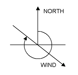
Figure: Definition of Wind field direction

Limited interval¶

The limited interval function allows the a specific time definition of when the boundary item is applied.

If a limited validity interval is to be applied to a boundary, then check ‘Use limited validity’. It is then necessary to define the start and end date & time of the validity period.

Scaling factor¶

The Scaling factor tab is used to apply a scale factor for the hydraulic load. This can be used to add a climate factor.

For 'Wind friction' boundary conditions, the scale factor for the wind velocity can be specified in the ‘Wind scaling factors’ editor.

Distributed weights¶

The 'Distributed weights' tab is used to compute and review the weights, used in combination with rainfall boundary conditions defined with the spatial extent type 'Grid distributed weights' (using input 2D radar data) or 'Data source location' (locating time series from their rain gauge coordinates). From this tab it is possible to check the distributed weights per catchment and adjust if desired.

With 'Grid distributed weights' boundaries, all catchments covered by the grid will be presented in the table. Catchments might be presented in several entries if multiple grid points cover its entirety.

There are two text fields which will display the most important data for the loaded boundary condition selected; grid file name and selected item name.

The table shows the connected grid cells (coordinates i and j) and the calculated weight percentage covering the catchment per grid cell.These percentages fractions should add up to a 100 per cent for each catchment.

The table is dynamic and shows the selected boundary condition data. It allows to insert new connecting grid cell by right clicking, or by typing a new catchment name in the last row.

The ‘Compute’ button allows to compute the weights for either all catchments or a selection of catchments, as well as for the new added grid points (not updated).

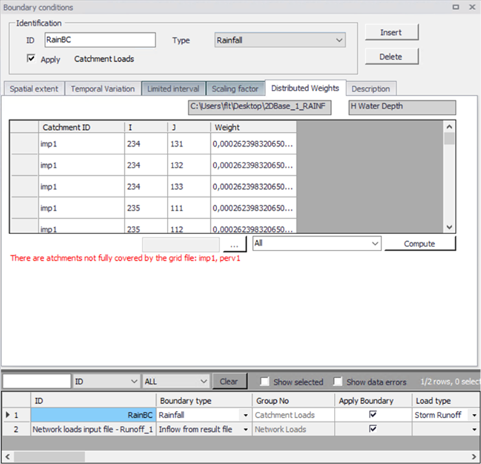
Figure: The ‘Distributed weights’ tab for a grid-distributed weights boundary condition

With 'Data source location' boundaries, the table is used only when the rainfall distribution type selected in the 'Simulation setup' editor (for the active simulation ID) is either 'Thiessen polygons weighting' or 'Inverse distance weighting'. The table will list all catchments having a positive weight associated to the active rainfall boundary conditions (catchments outside the Thiessen polygon surrounding the rain station, or beyond the search radius for the interpolation, are not listed in the table).

Text information above the table displays the weighting method selected in the active simulation ID, as well as the time series file name and item name used in the current boundary condition.

The 'Compute' button computes the weights for all the rainfall boundary conditions. The table can then be reviewed and updated if necessary. New rows can be added to the table by right-clicking, or by typing a new catchment name in the last row. If the tables of weights are left empty, the weights for all the rainfall boundary conditions will be computed when starting the simulation.

The 'Weights overview' button opens another table providing the complete list of weights, for each catchment and for each rainfall station.

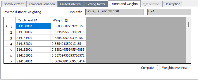
Figure: The 'Distributed weights' tab for a 'Data source location' boundary condition

During the simulation with 'Data source location' boundaries, the interpolated rain time series related to a catchment C is a weighted time series obtained from the various boundary time series \(Ts_{i}\) :

(7.1)

More details follows for the two available methods.

Inverse Distance Interpolation Method¶

Consider a plane with XY coordinates, the Catchment centroid coordinate \((X_{C}, Y_{C})\) and the sets of rain station measurements: \((Mx_{1}, My_{1})\) corresponding to the time series \(Ts_{1}\), \((Mx_{2}, My_{2})\) corresponding to the time series \(Ts_{2}\),…, \((Mx_{p}, My_{p})\) corresponding to the time series \(Ts_{p}\). Then the weight of each time series \(Ts_{j}\) is simply weighted proportionally to one over the square distance \(D(C, Ts_{j})\) between the catchment center \((X_{C}, Y_{C})\) and the measurement location \((Mx_{j}, My_{j})\):

(7.2)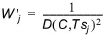

After computing all the weights for each measurement station, they need to be normalized so they sum up to 1:

(7.3)

The normalized weights are used to compute the interpolated rain of the catchments.

Thiessen Interpolation Method¶

The Thiessen (or Voronoi) interpolation is another simple way to decide the domain of influence of the measurements towards the catchments. A Thiessen polygon \(Tp_{i}\) is defined for each geolocated measurement time series \(Ts_{i}\), and it is roughly defined as the set of points in the plane for which the closest measurement location is the one defined by the geolocation of \(Ts_{i}\). Therefore, the edges of the Thiessen polygons correspond to equidistant lines between neighbor measurement locations. The overlapping of all these equidistant lines between all neighbor time series will define a set of polygons \(Tp_{1}, Ts_{2}, \ldots, Ts_{p}\).

Consider the n Catchments \(C_{1}, C_{2}, \ldots, C_{n}\) and the p measurement stations \(M_{1}, M_{2}, \ldots, M_{p}\). In the picture below, as example, 4 catchments and 6 stations:

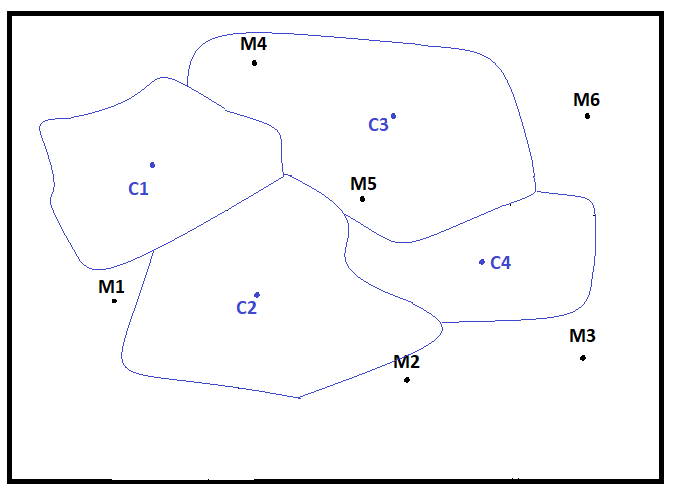
Figure: Example of catchments with geolocated rainfall stations

The stations \(M_{1}, M_{2}, \ldots, M_{p}\) and the surrounding box divide the plane into Thiessen/Voronoi polygons according to the distances to stations, as shown on the next figure.

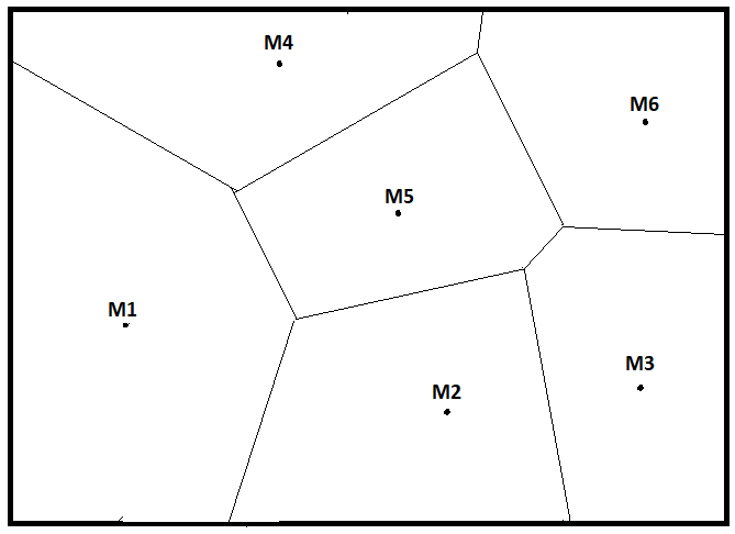
Figure: Thiessen polygons created from rainfall stations

The superposition of the Thiessen polygons divides the plane into areas where the closest station is the governing measurement which is consider for the polygon.

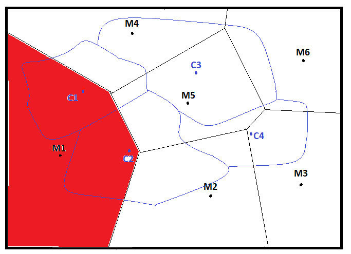
Figure: Thiessen polygon related to rainfall measurement station M1, in red

The weight related to catchment i and station j is the ratio between the Intersection of the catchment i and the Thiessen polygon j:

(7.4)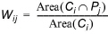

For the case of station 1 and catchment 1 the weight is the ration between the green area, and the sum of the green and brown areas:

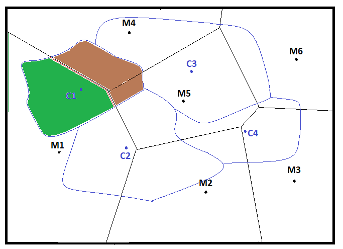
Figure: Thiessen weight calculation for catchment C1

Q/h Relation¶

The 'Q/h Relation' tab page is relevant for ‘River Q/h Relation’ boundary condition types. It is where the corresponding Q/h relation table for a ‘River Q/h Relation’ boundary condition is defined.

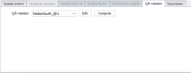
Figure: The Q/h Relation tab page relevant for River Q/h Relation boundary condition types

Select the appropriate Q/h relation table for the boundary condition from the ‘Q/h Relation’ dropdown list.

Use the ‘Edit’ button to access the ‘Curves and Relations’ editor, wherein one may edit or create various types of tabular data sets for the project.

Use the 'Compute' button to automatically compute the Q/h relation using the characteristics of the cross section located at the boundary location (a cross section must exist at this location before this tool can be used). The button opens the window below to control how to compute the Q/h relation.

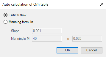
Figure: Automatic calculation of Q/h relations

H values in the Q/h relation are extracted from the processed data of the cross section whereas related Q values are computed either using the critical flow or the Manning formula. If the latter is chosen, the bed slope and Manning's value (Manning (M) or Manning (n)) must be specified.

In case the critical flow formula is used, Q is calculated from:

(7.5)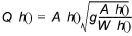

In case of uniform flow by Manning's formula, Q is calculated from:

(7.6)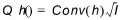

where:

Q(h) is the level dependent discharge
A(h) is the level dependent area (from Cross section processed data)
W(h) is the level dependent width (from Cross section processed data)
I is the bed slope
Conv(h) is the level dependent conveyance calculated as a function of the resistance type defined in cross section, in the Raw data tab, as described below.

If the resistance type is set to Relative Resistance:

(7.7)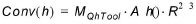

If the resistance type is set to Manning's M:

(7.8)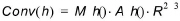

If the resistance type is set to Manning's n:

(7.9)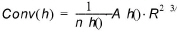

If the resistance type is set to Chezy or Darcy-Weisbach:

(7.10)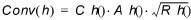

where:

\(M_{QhTool}\) is the Manning number defined in the 'Auto calculation of Q/h table' dialog
M(h), n(h) and C(h) are the respective resistance numbers extracted from the Resistance column in the cross sections Processed data.

Description¶

It is possible to provide a description of the boundary condition and load type using the Description field.

An 'Event ID' may also be associated with the boundary condition. The purpose of the event ID is to automatically filter the boundary conditions to include in a given simulation by selecting the corresponding event ID during the simulation execution, i.e. in the 'Simulation setup' editor. When a boundary condition is associated with a specific event ID, it will only be used in simulation setups defined with this same ID. The value 'Default (any event)' indicates that the boundary condition is not associated with any specific event and will be used in all simulations. It is possible to either use the pre-existing IDs available in the list or to add or edit IDs using the '…' option at the bottom of the list. See the Simulation Setup chapter for additional information.

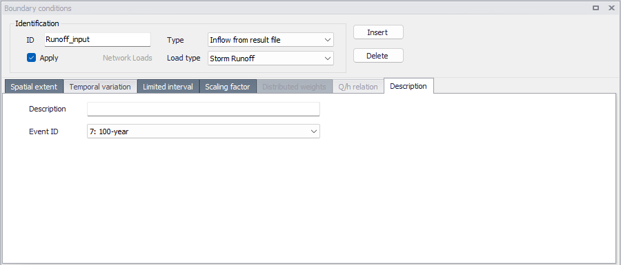
Figure: The 'Description' tab in the 'Boundary conditions' editor