Bridges

Working with bridges

'Bridge'-type structures are defined by one or more openings. The Bridges editor is therefore split into two parts:

• The main structure is defined in the primary table, in the left part of the editor. The main structure primarily stores information about the location of the bridge.
• The list of openings for the active main structure is defined in the secondary table, in the right part of the editor. Openings describe the various apertures under the bridge. Each opening is bound to the main structure on which it has been created, and a minimum of one opening is required for each main structure.

The figure illustrates an example of bridge containing multiple openings.

 

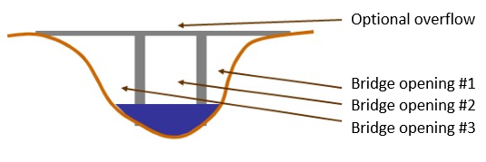
Figure: Example of bridge openings

A main structure may be added or removed from the map, or from the primary table on the left. Openings can only be controlled from the right part of the editor. Removing a main structure will remove all its openings as well.

 

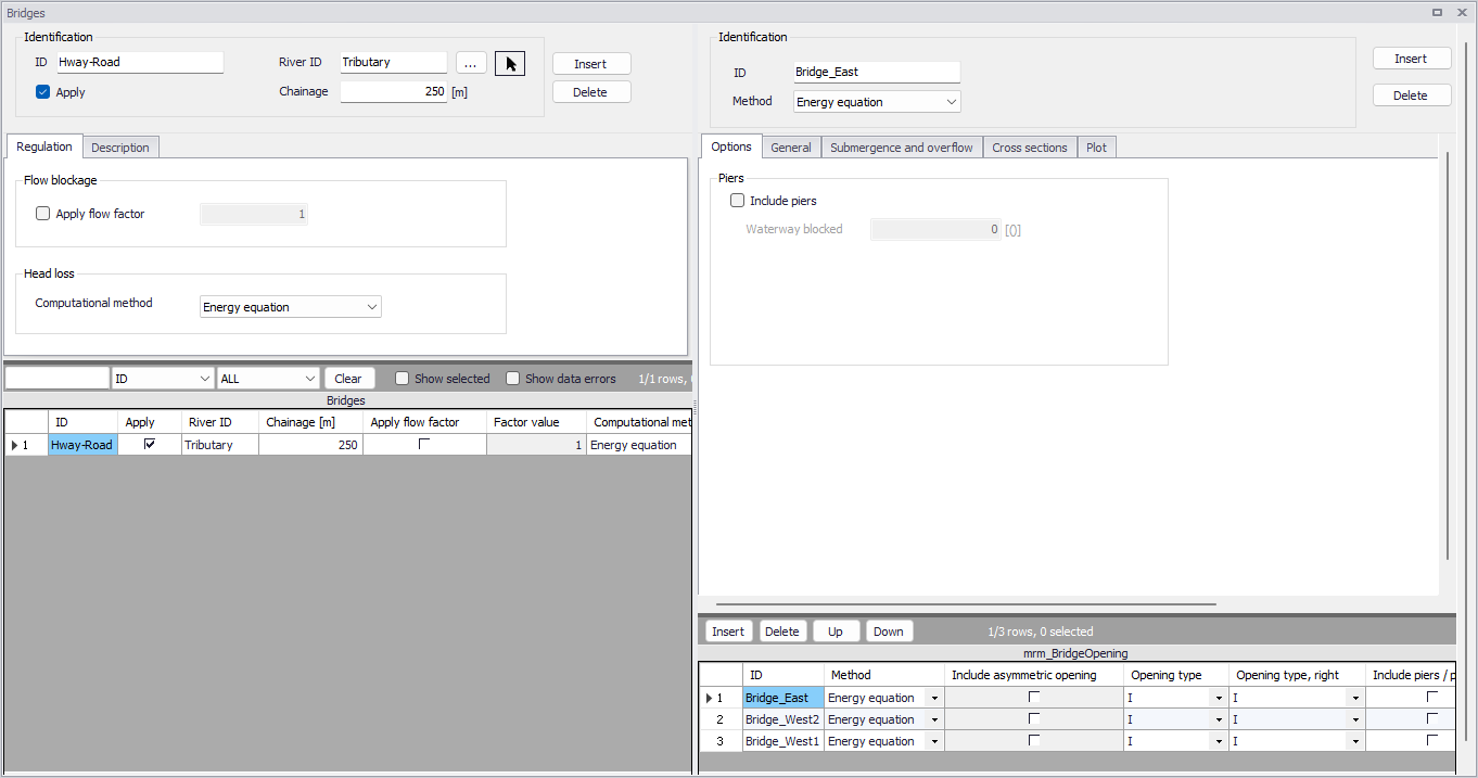
Figure: The Bridges editor accessed via the River Network setup group

Identification of the main structure

The Identification group holds basic information on bridges structures.

ID

Unique string identification for the bridge.

River ID

The ID of the river where the bridge is located. The River ID is automatically registered if the bridge is created via the Map. Use the button with an arrow, to select the location of the structure on the map: this will specify both the River ID and the Chainage of the structure.

Chainage

Chainage at which the bridge is located along the river.

Apply

This check box allows the user to toggle the Active status of the bridge on and off. The simulations will omit all bridges that are not active.

Regulation

Apply flow factor

When this option is active, the total discharge computed through the bridge (i.e. the sum of discharges through the various openings) is multiplied by a flow factor. This factor's value is specified in the Flow factor field. The factor is a dimensionless factor, and a value of 1 means that no change is applied to the computed discharge. A value lower than 1 can typically be used to describe the reduction of the flow through the structure due to obstacles, like debris, restricting the flow area in the structure.

Computational method

Two computational methods are available:

• Energy equation: with this method, the flow through the structure is solved using the energy equation, in order to compute the discharge in the structure as a function of the head loss factors. The computed discharge is then applied at the calculation point. . This is the preferred option in case there are big changes in cross sections before and after the structure, or if the flow area of the structure is much less than that of the river.
• Shallow water equation: with this method, the flow through the structure is solved adding a head loss term to the shallow water equation (Saint-Venant momentum equation), this term being a function of the head loss factors. With this method, the same equation is applied at structures' locations as at other regular calculation points (without structures). This ensures a continuity of the results between the upstream / downstream reaches and the structure, e.g. also including a bed friction between the upstream and downstream cross sections of the structure. Additionally, this method also enforces the use of velocity in upstream and downstream cross sections to compute the head loss, instead of using the velocity in the structure. This option is mainly designed for scenarios where the structure creates little or no head loss for low water levels, as e.g. for an overarching bridge. See the "Head loss mode" in the MIKE 1D reference manual, for more information.

Note

When the flow through the structure becomes supercritical, the applied method is always the Energy equation. Besides, the 'Shallow water equation' method cannot be applied for structures located on rivers of type 'Structure link'. When several structures exist at the same location, if any of them uses the Shallow water equation method, then all other structures at the same location will also apply the same equation no matter the selected method in their properties.

Description

Use the Description tab to add free text descriptions for bridges structures (Figure 3.77). It offers options for providing model management information, as well as attributes for quick model data query.

 

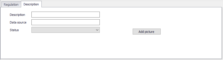
Figure: The Description tab on the Bridges structures editor

• Description: Free text description for the tabulated structures.
• Data source: Free text describing data source for tabulated structures data.
• Status: Project-defined status information that may be used for model build management or e.g. model data query. Pre-defined codes are contained in the Status Code editor which may be accessed via the ellipsis button from the Status dropdown menu.
• Add picture: Option for adding images associated with the tabulated structure.

Identification of the opening

This Identification group holds basic information on the bridge's opening.

ID

Unique string identification for the opening.

Method

The method controls the equation applied to describe the free surface flow through the opening. The available methods can be divided into pure free flow methods and methods which may be combined with submergence/overflow methods. The pure free flow methods can be further subdivided into methods for piers and methods for arches. The choice of method should be based on the assumptions for the different methods and the requirements of the modelling. The available methods are:

• Energy equation: a standard step method where a backwater surface profile determination is used to calculate the discharge through the opening. The method takes the contraction and expansion loss for bridges of arbitrary shape into account. The method assumes subcritical flow and may default to critical flow for steep water surface gradients.
• FHWA WSPRO: the Federal Highway Administration (FHWA) WSPRO method is based on the solution of the energy equation. Contraction loss is taken into account through the calculation of an effective flow length. Expansion losses are determined through the use of numerous experimentally based tables. The method takes the effect of eccentricity, skewness, wingwalls, embankment slope etc. into account through the use of these tables.
• USBPR: the US Bureau of Public Roads (USBPR) method estimates free surface flow assuming normal depth conditions. The method is based on experiments and takes the effect of eccentricity, skewness and piers into account.
• Yarnell piers: an equation derived from experiments for normal flow conditions in the subcritical flow range. The effect of piers is handled through the use of adjustment factors.
• Nagler piers: an orifice type of flow description with the effect of the piers taken into account through an adjustment factor.
• Hydraulic Research arch: the Hydraulic Research method is based on laboratory experiments of both single and multi-spanned arch bridges in rectangular channels. The method uses tables describing the relationship between the blockage ratio, the downstream Froude number and the upstream water level.
• Biery and Delleur arch: an orifice type of equation is used to describe the discharge through the opening. The equation is derived under the assumption of a rectangular channel and is based on a single span arch opening. Multiple arch openings are handled by a simple multiplication factor.

Include asymmetric opening

Used for individual definition of left and right abutments' properties. When this option is active, most of the opening's parameters have to be defined separately for the left and for the right side. This option is only available with the FHWA WSPRO method.

Opening type

For the FHWA WSPRO method, the opening type describes the type of embankment and abutment, through four different types: I, II, III and IV.

 

Figure: Definition sketch of opening type I (vertical embankments and vertical abutments, with or without wingwalls) (after Matthai)

 

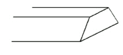
Figure: Definition sketch of opening type II (sloping embankments without wingwalls) (after Matthai)

 

Figure: Definition sketch of opening type III (sloping embankments and sloping abutments; spillthrough) (after Matthai)

 

Figure: Definition sketch of opening type IV (sloping embankments and vertical abutments with wingwalls) (after Matthai)

Options

Additional options may be added to the free surface flow calculation. Available options depend on the selected method. To include an option, simply tick the corresponding box.

Most of the options are taken into account through the use of adjustment factors defined in tables. It is possible to either use the default tables or use custom tables.

Piers and piles.

This option may be used to include the effect of piers and piles on the free surface flow calculation.

Waterway blocked

The proportion of the waterway blocked by piers/piles.

Type

For the FHWA WSPRO method, two types are available:

• Piers
• Piles.

For the USBPR method, the following types of piers are available:

• Single cylinder
• Twin cylinder 1
• Twin cylinder 2
• Series of cylinder
• Single squared
• Twin squared 1
• Twin squared 2
• Series of squared
• Semi-circular
• Series of I-formed.

Use custom table

When this option is unchecked, the simulation uses the default loss tables for piers and piles. When checked, the simulation uses user-defined tables, which are selected in the corresponding fields, using the ellipsis button.

For the FHWA WSPRO method with type 'Piers', the table must be defined in the 'Curves and relations' editor, and with a type 'Bridge FHWA WSPRO piers'. For the FHWA WSPRO method with type 'Piles', two table must be defined:

• The expected type for the first / upper table depends on the opening type. For the opening type I, the table must be defined in the 'Curves and relations' editor, and with a type 'Bridge FHWA WSPRO piles type I'. For the other opening types, the table must be defined in the 'Two-dimensional tables' editor, and with type 'Bridge FHWA WSPRO piles' to store the values of the adjustment factor kp (for j=0.1).
• The second / lower table must be defined in the 'Curves and relations' editor, and with type 'Bridge FHWA WSPRO piles table 2'

For the USBPR method, the table must be defined the 'Curves and relations' editor, and with a type 'Bridge USBPR piers'.

Please refer to the reference manual for descriptions of variables used in the tables.

Skewness

Skewness can be applied when the abutments are not perpendicular to the flow direction.

Angle

Angle describing the orientation of abutments.

When this option is unchecked, the simulation uses the default loss table for skewness. When checked, the simulation uses a user-defined table, which is selected in the corresponding field, using the ellipsis button.

The table must be defined in the 'Curves and relations' editor, and with a type 'Bridge USBPR skewness'.

Please refer to the reference manual for descriptions of variables used in the table.

Eccentricity

Eccentricity can be applied when the bridge opening is eccentrically located in the river.

When this option is unchecked, the simulation uses the default loss table for eccentricity. When checked, the simulation uses a user-defined table, which is selected in the corresponding field, using the ellipsis button.

For the FHWA WSPRO method, the table must be defined in the 'Curves and relations' editor, and with a type 'Bridge FHWA WSPRO eccentricity'. For the USBPR method, the table must be defined in the 'Two-dimensional tables' editor, and with a type 'Bridge USBPR eccentricity' to store the values of the parameter ke.

Please refer to the reference manual for descriptions of variables used in the table.

Spur dykes

This option may be used to include the effect of spur dykes on the free surface flow calculation.

When this option is unchecked, the simulation uses the default loss tables for spur dykes. When checked, the simulation uses user-defined tables, which are selected in the corresponding fields, using the ellipsis buttons.

For the opening types I, II and IV, only one table is used: it must be defined in the 'Curves and relations' editor, and with a type 'Bridge FHWA WSPRO spur dyke'. For the opening type III, two tables are used:

• The first / upper table must be defined in the 'Two-dimensional tables' editor, and with type 'Bridge FHWA WSPRO spur dyke III'. It stores values for the kd parameter.
• The second / lower table must be defined in the 'Two-dimensional tables' editor, and also with type 'Bridge FHWA WSPRO spur dyke III', but this one stores values for the ka parameter.

Please refer to the reference manual for descriptions of variables used in the tables.

Length

The length of the spur dyke.

Type

The type of the spur dyke, which can be either straight or elliptical.

Angle

The angle, for an elliptical spur dyke.

Offset

The offset, for a straight spur dyke.

General

The parameters available here control the free surface flow equations applied for the active opening. The number of parameters depends on the selected method.

Roughness type

Defines the type of roughness value specified for the opening. The type can be either Manning's M or Manning's n.

Roughness value

The value for the roughness on the bridge structure.

This roughness value will per default apply all along the bridge's cross sections. However, if these cross sections have markers 'Left abutment' and 'Right abutment' specified, then it is assumed that the part of the cross sections in-between represents the river bed, and the roughness applied between these markers is obtained from the roughness applied to the upstream and downstream cross sections. In this case, the roughness value specified for the opening only applies from the left extent of the bridge's cross section to 'Left abutment' marker, and from 'Right abutment' marker to the right extent of the bridge's cross section.

Ratio

Selects between the channel contraction ratio (m=1-M) or bridge opening ratio (M) as parameter in the various tables.

Waterway length

Length of the waterway in the flow direction.

Level of waterway length

The level at which the waterway length is measured.

Contraction loss coef.

The contraction loss factor.

Expansion loss coef.

The expansion loss factor.

Opening width

For an arch: opening width at the arch spring line (b, in figure below). For piers: total opening width between the piers.

 

Figure: Geometrical description of an arch

Type of piers

Describes the shape of the piers:

• Squared
• Semi-circular
• 90-degree triangular
• Twin cylinder without diaphragm
• Twin cylinder with diaphragm
• Lens-shaped
• Ten pile trestle bent (only available for Yarnell piers)

The selected type of piers is only used when applying predefined tables of coefficients. When working with custom tables instead, the type of piers is not used.

Number of arches

The number of arches in the opening.

Level of bottom of arch curvature.

Level of arch spring line, shown on the figure above.

Level of top of arch curvature

Level of upper most point in the arch, shown on the figure above.

Radius of arch curvature

Radius of the arch (r, in the figure above).

Use custom table

When this option is unchecked, default loss factor tables are used in the simulation. When checked, a user-defined table may be used, which is selected in the corresponding field, using the ellipsis button.

For the Yarnell piers method, the table must be defined in the 'Curves and relations' editor, and with a type 'Bridge Yarnell piers'. For the Nagler piers method, the table must be defined in the 'Curves and relations' editor, and with a type 'Bridge Nagler piers'. For the Hydraulic Research arch method, the table must be defined in the 'Two-dimensional tables' editor, and with a type 'Bridge Hydraulic Research arch' to store values for the parameter H1/Y4. For the Biery and Delleur arch method, the table must be defined in the 'Two-dimensional tables' editor, and with a type 'Bridge Biery and Delleur arch' to store the values for the coefficient of discharge.

Free surface flow

This tab contains additional geometrical parameters for the FHWA WSPRO and USBPR methods. When working with asymmetric openings, these parameters must be specified for the left and right side, respectively.

Use custom table

When this option is unchecked, the simulation uses the default loss table for the related item. When checked, the simulation uses a user-defined table, which is selected in the corresponding field, using the ellipsis button. In this user-defined table, it is possible to add more rows and sometimes more columns, and edit the values.

For the FHWA WSPRO method, the following custom tables may be used:

• Base coefficient: for opening type I, the table must be defined in the 'Curves and relations' editor and with a type 'Bridge FHWA WSPRO base coef. type I'. For opening types II, III and IV, the table must be defined in the 'Two-dimensional tables' editor, respectively with type 'Bridge FHWA WSPRO base coef. type II', 'Bridge FHWA WSPRO base coef. type III' and 'Bridge FHWA WSPRO base coef. type IV' to store the values of the base coefficient C.
• Entrance rounding: the table must be defined in the 'Curves and relations' editor, and with a type 'Bridge FHWA WSPRO entrance'.
• Froude number: the table must be defined in the 'Curves and relations' editor, and with a type 'Bridge FHWA WSPRO Froude'.
• Average depth: the table must be defined in the 'Curves and relations' editor, and with a type 'Bridge FHWA WSPRO depth' to store the values of the parameter ky.
• Abutment: the table must be defined in the 'Curves and relations' editor, and with a type 'Bridge FHWA WSPRO abutment' to store the values of the parameter kx.
• Wingwalls: the table must be defined in the 'Curves and relations' editor, and with a type 'Bridge FHWA WSPRO wingwall'.

For the USBPR method, the following custom tables may be used:

• Base coefficient: the table must be defined in the 'Curves and relations' editor, and with a type 'Bridge USBPR base coefficient'.
• Velocity distribution coefficient: the table must be defined in the 'Two-dimensional tables' editor, and with a type 'Bridge USBPR velocity distribution' to store the values of the parameter Alpha2.

Please refer to the reference manual for descriptions of variables used in the tables for the various methods.

Type (Base coefficient)

Three types of openings are available with the USBPR method:

• 90\(^\circ\) wingwall
• 45\(^\circ\) wingwall
• Spillthrough

Type (Entrance rounding)

For opening type I with FHWA WSPRO method, two types of entrance rounding are available:

• Corner
• Wingwall.

 

Figure: Rounding type for opening type I (Left: corner; Right: wingwall)

Radius (Entrance rounding)

Radius of the corner (r, in the figure above).

Width (Entrance rounding)

Width of the wingwall (W, in the figure above).

Angle (Entrance rounding)

Angle of the corner (Angle, in the figure above).

Embankment slope

The slope of the embankment for opening types II, III, and IV with FHWA WSPRO method. For example, use a value 2 for a 1:2 slope.

Angle (Wingwalls)

Angle of the wingwall for opening type IV with FHWA WSPRO method.

Submergence and overflow

Under the Submergence and overflow tab, it is possible to optionally include either submergence, or submergence and overflow.

These options are only available in combination with the Energy equation, FHWA WSPRO or USBPR method for free surface flow calculation.

Submergence

Method

The method controls the equation applied to describe the submerged flow through the opening. The choice of method should be based on the assumptions for the different methods and the requirements of the modelling. The available methods are:

• FHWA WSPRO: the Federal Highway Administration (FHWA) WSPRO method for pressure flow is based on two orifice equation descriptions. One for situations when the orifice is submerged downstream and a modified equation for situations when only the upstream part of the orifice is submerged.
• Energy equation: the flow under the opening is determined through a standard backwater step method. The flow is assumed to be in the subcritical range and thus the method may default to critical flow. Both contraction and expansion losses are taken into account.
• Culvert: a standard culvert description may be chosen for submergence flow, where the culvert is specified in the 'Culverts' editor. The culvert is only active if submergence occurs.

Discharge coefficient

The discharge coefficient in the FHWA submergence equation.

Use custom table

When this option is unchecked, the simulation uses the default table for coefficient of discharge. When checked, the simulation uses a user-defined table, which is selected in the corresponding field, using the ellipsis button.

The table must be defined in the 'Curves and relations' editor, and with a type 'Bridge FHWA WSPRO submergence'.

Please refer to the reference manual for descriptions of variables used in the table.

Bridge soffit level

The soffit (underside) level of the opening.

Contraction loss

The contraction loss coefficient.

Expansion loss

The expansion loss coefficient.

Culvert

The ID of the selected culvert to be used, from the list of valid structures in the 'Culverts' editor. The culvert must be located on the same river and the same chainage as the bridge.

Overflow

The method controls the equation applied to describe the flow over the bridge. The choice of method should be based on the assumptions for the different methods and the requirements of the modelling. The available methods are:

• FHWA WSPRO: the Federal Highway Administration (FHWA) WSPRO method is based on a weir equation taking tail water submergence into account through the use of a submergence coefficient. The method may be used for both gravel and paved surfaces.
• Energy equation: the flow over the bridge is determined through a standard backwater step method. The flow is assumed to be in the subcritical range and thus the method may default to critical flow.
• Weir: a standard weir description may be chosen for overflow, where the weir is specified in the 'Weirs' editor. The weir is only active if overflow occurs.

Bridge deck level

The deck (underside) level for the opening.

Length

The length of top of embankment in the flow direction.

Use custom tables

When this option is unchecked, the simulation uses the default tables for coefficients of discharge and for the submergence factor. When checked, the simulation uses user-defined tables, which are selected in the corresponding fields, using the ellipsis buttons.

The tables must be defined in the 'Curves and relations' editor. The table for discharge coef. #1 must have a type 'Bridge FHWA WSPRO overflow cf1'. The table for discharge coef. #2 must have a type 'Bridge FHWA WSPRO overflow cf2'. The table for the submergence factor must have a type 'Bridge FHWA WSPRO overflow kt'.

Please refer to the reference manual for descriptions of variables used in the tables.

Surface

The surface of the top of the bridge, required when using default tables, and which can be of type:

• Paved
• Gravel.

Weir

The ID of the selected weir to be used, from the list of valid structures in the 'Weirs' editor, from the river network. The weir must be located on the same river and the same chainage as the bridge.

Cross sections

In the Cross sections tab, it is required to specify the geometry of the bridge opening, on both its upstream and its downstream side. The corresponding bridge's cross sections should describe the bottom of the opening as well as its lateral walls, and are used for the free surface flow calculation. When submergence and overflow are included, the levels of submergence and overflow are specified in the Submergence and overflow tab, and therefore don't have to be included in the bridge's cross sections.

The upstream and downstream bridge's cross sections are illustrated on Figure 6.29, representing a plan view of the bridge, respectively as sections 2 and 3. Cross sections 1 and 4 are the closest cross sections defined in the Cross sections editor.

 

Figure: Location of upstream and downstream cross sections

The location of the cross sections outside the bridge (as defined in the Cross sections editor from the tree view) should be so that any potential contraction or expansion loss is taken into account. In other words, the optimal location is where the stream lines are parallel prior to a contraction and post a possible expansion. As a rule of thumb, the distance between the bridge and the cross sections should be in the order of one opening width.

Upstream section, free surface flow

The upstream cross section of the opening is defined in a table, which provides a list of points describing the topography along the lateral walls and the bottom of the opening.

The 'S' column provides the horizontal distance of each point along the cross section, from the left end of the cross section. Note that the S-values are compared to the S-values of the upstream cross section (defined in the 'Cross sections' editor), and it is therefore important that S-values are consistent between these cross sections.

The 'Z' column provides the elevation of the points.

The 'Roughness' column provides the relative resistance in the cross section point. A factor 1 corresponds to the resistance value specified in the General tab.

The 'Marker' column may optionally contain the following markers:

• 'Left extent': defines the left extent of the active part of the cross section used for the calculation. All points of the cross section located to the left of this marker are ignored. If this marker is not defined in the cross section, it is assumed that left extent corresponds to the first point in the table.
• 'Left abutment': defines the horizontal position of the bottom of the left wall of the opening.
• 'Right abutment': defines the horizontal position of the bottom of the right wall of the opening.
• 'Right extent': defines the right extent of the active part of the cross section used for the calculation. All points of the cross section located to the right of this marker are ignored. If this marker is not defined in the cross section, it is assumed that right extent corresponds to the last point in the table.

When markers 'Left abutment' and 'Right abutment' are defined in the cross section, it is assumed that the part of the cross section between these two markers corresponds to the natural river bed, and in this case the roughness applied between these markers is obtained from the upstream and downstream cross sections. If these markers are not defined, the roughness value specified in the General tab will be uniformly applied along the bridge's cross section.

The buttons above the table can be used to insert, delete and re-order lines in the table.

Datum

A datum value may be entered here. The datum is added to all Z values in the table. The datum is normally used for adjusting the levels of the cross sections such that they conform to a specific reference datum in the model area.

Copy upstr. section

The button 'Copy upstr. section' fills in the table, by copying the S, Z and roughness values from the first cross section located upstream of the bridge. This allows to easily obtain the geometry of the upstream cross section, and manually edit this cross section afterwards to describe the geometry of the bridge.

Use custom sub-cross section

When the main structure contains multiple openings, the entrance loss upstream and downstream of each opening is computed using a sub-part of the upstream cross section (defined in the 'Cross sections' editor), and not using the full width of the upstream cross section. The upstream sub-cross section represents the part of the cross section where the water flows towards the active opening.

When the option 'Use custom sub-cross section' is unchecked, the upstream sub-cross section is defined automatically, based on geometrical considerations only. When the option is checked, the position of the upstream sub-cross is manually defined between 'From S value' and 'To' S-value.

From S value

This value represents the left horizontal extent of the upstream sub-cross section. This S value refers to the S value specified in the raw data table of the upstream cross section, defined in the Cross sections editor.

To S value

This value represents the right horizontal extent of the upstream sub-cross section. This S value refers to the S value specified in the raw data table of the upstream cross section, defined in the Cross sections editor.

Downstream section, free surface flow

The downstream cross section of the opening may either be defined as a copy of the upstream cross section of the bridge, in which case elevations are corrected using a longitudinal slope, or defined with its own table.

Cross section

This controls the way the downstream cross section of the bridge is defined:

• Same as upstream: the downstream cross section of the bridge is defined with data from the upstream cross section, but with a correction of elevations to take the longitudinal slope into account.
• User-defined section: the downstream cross section of the bridge is defined in its own table. Please refer to the description of the table used for the upstream cross section for more details.

Slope

The slope between the upstream and the downstream cross sections of the bridge.

A datum value may be entered here when the downstream cross section of the bridge is defined in its own table. The datum is added to all Z values in this table. The datum is normally used for adjusting the levels of the cross sections such that they conform to a specific reference datum in the model area.

Copy downstr. section

The button 'Copy downstr. section' fills in the table, by copying the S, Z and roughness values from the first cross section located downstream of the bridge. This allows to easily obtain the geometry of the downstream cross section, and manually edit this cross section afterwards to describe the geometry of the bridge.

Use default downstream sub-cross section

When the main structure contains multiple openings, the exit loss downstream of each opening is com-puted using a sub-part of the downstream cross section (defined in the 'Cross sections' editor), and not using the full width of the downstream cross section. The downstream sub-cross section represents the part of the cross section where the water flows from the active opening.

When the option 'Use custom sub-cross section' is unchecked, the downstream sub-cross section is defined automatically, based on geometrical considerations only. When the option is checked, the position of the downstream sub-cross is manually defined between 'From S value' and 'To' S-value.

This value represents the left horizontal extent of the downstream sub-cross section. This S value refers to the S value specified in the raw data table of the downstream cross section, defined in the Cross sections editor.

This value represents the right horizontal extent of the downstream sub-cross section. This S value refers to the S value specified in the raw data table of the downstream cross section, defined in the Cross sections editor.

Plot

To help ensuring that the geometry of the bridge is properly defined, the bridge's cross sections are shown and are compared to its upstream and downstream cross sections. On this plot, the horizontal axis shows the X-coordinates from the upstream cross section. The downstream cross section is then shifted so that its marker 2 is aligned with the marker 2 from the upstream cross section. The bridge's cross sections are also centered around this marker 2, but can be moved horizontally using the value 'Horizontal offset from marker 2'.

Note

This horizontal offset value is only used for the visualization purpose and has no impact on the simulation.