2D Surface Roughness
The way in which surface roughness is applied to the model can be specified in four different ways:
- Uniform
- Varying in Domain
- Varying in Domain and Time
- Varying in domain and flow dependent
Uniform
When a Uniform roughness type is selected, the roughness formula must be selected (Manning M, Manning n or Chezy C) and one roughness value specified. This value will be applied to the entire 2D domain.
Varying in Domain
To define spatially varying 2D roughness, the following sources of information can be used:
MIKE+ 2D Surface Roughness Layer
This option enables a roughness layer to be graphically defined in the "Map" view using the tools available in the "2D overland" ribbon.
Steps to define roughness polygons:
- Select the Target layer as "2D surface roughness"
- Click on "Create" and define polygons. Utilise the various editing tools to refine the polygons if necessary. Tip: specify a default roughness formula and value in the 2D surface roughness table to automatically populate the values of a polygon as soon as it is digitised.
- In the 2D roughness table, the digitised polygons will be listed. Specify the roughness values for each of these polygons, and prioritise them using the up and down buttons (important if there are overlaps)
- To access predefined roughness values specified in the Materials table (Setup | Tables | Materials), specify the Value type as "Material" and select the Material type from the drop-down list.
- To define specific roughness values, select the value type "Local" and input the value in the "Roughness" column
- Where the model domain is not covered by the roughness polygons the default value will be used in this area.
Clicking on "Review roughness file on map" will build a 2D Surface Roughness *.DFS2 or *.DFSU file and add the layer to the map. This layer will also be saved in your project directory for use in the simulation. This file will also be created when starting the simulation, if it doesn't exist in the project directory of if input data have been modified.
Background Layer of Individual Polygons
Utilize predefined information to define the 2D surface roughness. E.g. from Shape files, Tab files or Raster text files.
Steps to define the surface roughness details:
- Layer: Select the appropriate layer that has already been loaded into the MIKE+ interface as a background layer (available in the drop-down list) or browse to a saved file.
- Item: Select the field in the layer that contains roughness values
- Roughness formula: Select the formula to be used - Manning (M), Manning (n), Chezy (C)
- Unit: Depending on the formula, select the relevant SI or US unit
- Default roughness value: Value to be used if no roughness value exists in the layer
Clicking on "Review roughness file on map" will build a 2D Surface Roughness *.DFS2 file and add the layer to the map. This layer will also be saved in your project directory for use in the simulation. This file will also be created when starting the simulation, if it doesn't exist in the project directory of if input data have been modified.
2D File
Use a previously defined *.DFS2 or *.DFSU file with "Mannings M", "Mannings n" or "Chezy No" item type as the 2D surface roughness.
If a *.DFSU file is used, piecewise constant interpolation is used to map the data. If a DFS2 file is used, bilinear interpolation is used to map the data. If the input data file contains a single time step, this field is used. In the case where the file contains several time steps, e.g. from the results of a previous simulation, the actual starting time of the simulation is used to interpolate the field in time. Therefore, the starting time must be between the start and end time of the file.
Background Layer of Land Cover
The 'Background layer of land cover' option allows defining the surface roughness as a function of land cover, i.e. per land cover type. A polygon layer must be selected to define the land cover, in which the polygons are grouped by category (land cover type). Three types of file format can be used for defining the land cover types:
- Shape file
- DFS2 or DFSU file
- XYZ file
For XYZ files and shape files, the land cover zones are defined as the closed region within a number of polygons. For dfs files, the zones are defined by a map identifying the location of the different zones. Each land cover type is identified by an integer number larger than zero. If an element from the 2D domain belongs to more than one polygon in the XYZ file or the shape file, the information from the last polygon read from the file is applied. If there are overlapping zones with the buildings and road zones (from the 2D infrastructures editor), the priority is first given to the building zones, then to the road zones and finally to the land cover zones.
For dfs files, the value should be zero in areas with no local infiltration zone in a dfs file.
For XYZ files, the data in the file must be formatted as ASCII text in five columns with the two first columns giving the x-and y-coordinates of the points. The third column represents connectivity. The connectivity column is used to define arcs. All points along an arc - except the last point - shall have a connectivity value of 1 and the last point shall have a connectivity value of 0. The fourth column contains the z-value at the point, which is unused for land cover layers. Finally, the fifth column contains the zone number, corresponding to the land cover type.
In the 'Land cover layer' section , the following needs to be specified:
- Layer: The source layer defining the land cover zones
- Item: For a shape file or dfs file, this is the attribute or item in the file containing the integer number, used to identify the land cover type each polygon belongs to.
- Map projection: For a XYZ file, this is the map projection in which the XY coordinates in the file are defined.
In the 'Roughness values' section, the roughness formula must be selected (Manning M, Manning n or Chezy C), and the roughness values must be specified for each zone in the table. The list of zones is made of the list of land cover types plus the list of road zones and / or buildings zones eventually selected in the 2D infrastructures editor. The land cover ID for these zones is editable. A default roughness value must also be supplied, which is applied in areas not covered by any of the previous zones.
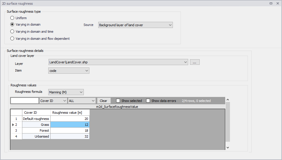
Figure: Defining roughness values for land cover zones
Varying in Domain and Time
The 2D surface roughness can be specified to vary both spatially and in time. In this case the user must select a previously defined *.DFS2 or *.DFSU, that varies in time. Browse to the file or if the file has been loaded as a background layer in MIKE+ it will be available from the drop-down list. Open the file via the "View" button to interrogate and edit the file. The item type for the values in this file must be "Mannings M", "Mannings n" or "Chezy No".
If a *.DFSU file is used, piecewise constant interpolation is used to map the data. If a DFS2 file is used, bilinear interpolation is used to map the data. If the data is varying in time the data must cover the complete simulation period. The time step of the input data file does not however need to match the time step of the hydrodynamic simulation. A linear interpolation will be applied if the time steps differ.
When using an external file (water level or water depth and velocity), the area in the data file must cover the model area. If a *.DFSU file is used, piecewise constant interpolation is used to map the data. If a DFS2 file is used, bilinear interpolation is used to map the data. Delete values (used in empty elements of the file) will be ignored and the value will be interpolated only from existing data.
Varying in Domain and Flow Dependent
The 'Varying in domain and flow dependent' option allows defining the surface roughness as a function of the flow on the surface (water depth or flux) and as a function of land cover, i.e. per land cover type. A polygon layer must be selected to define the land cover, in which the polygons are grouped by category (land cover type). Three types of file format can be used for defining the land cover types:
- Shape file
- .DFS2 or .DFSU file
- XYZ file.
For XYZ files and shape files, the land cover zones are defined as the closed region within a number of polygons. For dfs files, the zones are defined by a map identifying the location of the different zones. Each land cover type is identified by an integer number larger than zero. If an element from the 2D domain belongs to more than one polygon in the XYZ file or the shape file, the information from the last polygon read from the file is applied. If there are overlapping zones with the buildings and road zones (from the 2D infrastructures editor), the priority is first given to the building zones, then to the road zones and finally to the land cover zones.
For dfs files, the value should be zero in areas with no local infiltration zone in a dfs file.
For XYZ files, the data in the file must be formatted as ASCII text in five columns with the two first columns giving the x-and y-coordinates of the points. The third column represents connectivity. The connectivity column is used to define arcs. All points along an arc - except the last point - shall have a connectivity value of 1 and the last point shall have a connectivity value of 0. The fourth column contains the z-value at the point, which is unused for land cover layers. Finally, the fifth column contains the zone number, corresponding to the land cover type.
In the 'Land cover layer' section , the following needs to be specified:
- Layer: The source layer defining the land cover zones
- Item: For a shape file or dfs file, this is the attribute or item in the file containing the integer number, used to identify the land cover type each polygon belongs to.
- Map projection: For a XYZ file, this is the map projection in which the XY coordinates in the file are defined.
In the 'Roughness values' section, the roughness curves must be specified for each zone in the table. The list of zones is made of the list of land cover types plus the list of road zones and / or buildings zones eventually selected in the 2D infrastructures editor. The land cover ID for these zones is editable. A default roughness curve must also be supplied, which is applied in areas not covered by any of the previous zones. For each zone, the data to be specified are:
- Function of: Controls whether the Manning number is specified as a function of the water depth or as a function of the flux.
- Roughness curve: The curve defining the Manning number as a function of the depth or flux. When the roughness is defined as a function of water depth, the valid curve types are either 'Depth dependent Manning (M)' or 'Depth dependent Manning (n)'. When the roughness is defined as a function of flux, the valid curve types are either 'Flux dependent Manning (M)' or 'Flux dependent Manning (n)'.
The 'Create curves' button can be used to create curves with default values for each of the zones. The curve data are accessed via the Curves and Relations editor.
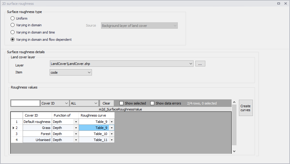
Figure: Defining flow-dependent roughness values for land cover zones
Scientific Description
The 2D flow model uses either a Chezy number or a Manning number (M) assigned to each grid cell/element cell to describe the roughness (bed resistance). Note, that the Manning number used here is the reciprocal value of the Manning´s n described in some textbooks.
The bed resistance, t, is determined by a quadratic friction law
(3.5) 
where \(c_{f}\) is the drag coefficient, u is the velocity and \(r_{0}\) is the density of the water.
The drag coefficient can be determined form the Chezy number, C, or Manning number, M.
(3.6) 
(3.7) 
where h is the total water depth and g is the gravitational acceleration.
The units of Chezy numbers and Manning numbers are \(\text{m}^{1/2}/\text{s}\) and \(\text{m}^{1/3}/\text{s}\) respectively.
The relation between the Manning number and the bed roughness length, \(k_{s}\), can be estimated using the following
(3.8) 
Recommended Values
If the relative variation of the water depth is considerable then using variation in Manning's numbers are recommended. Values for Manning's M in the range 10-40 \(\text{m}^{1/3}/\text{s}\) are normally used.
If Chezy numbers are applied, a model calibration can normally be achieved with values in the range 30 - 50 \(\text{m}^{1/2}/\text{s}\).
Because of the definition of the resistance numbers the following applies when using Manning's M:
- Using a smaller resistance number increases the bed resistance
- Using a greater resistance number decreases the bed resistance.
Remarks and Hints
If the boundary conditions at one of your boundaries are inaccurate and you therefore have stability problems (blow-ups) at this boundary, you can specify a small band (2 to 4 grid lines) with a very high resistance. Manning numbers in the range 5 -10 \(\text{m}^{1/3}/\text{s}\) have been applied successfully. However, this method should only be used if it is impossible to improve the boundary conditions. Furthermore, the simulation results in the area around the small resistance numbers should be used with caution.
Because \(h^{1/6}\) is calculated for each grid point and at each time step when the Manning formulation is selected rather than the Chezy formulation, the computational time is increased.