Multi-Species Analysis¶

Standard EPANET-based water quality component is limited to tracking the transport and fate of just a single chemical species, such as fluoride used in a tracer study or free chlorine used in a disinfectant decay study. This multi-species analysis describes a water quality extension that allows it to model any system of multiple, interacting chemical species.

Many water quality problems in distribution systems can only be analyzed by using a multi-species approach. Consider the following descriptive examples:

Free chlorine disinfectant is lost in bulk solution due mainly to oxidation-reduction reactions involving HOCl and OCl- and natural organic matter (NOM). The NOM itself is a heterogeneous mixture of organic compounds (e.g., humic and fulvic acids) of varying chemical characteristics. Current single-species models, however, must model free chlorine loss under the assumption that all other reactants are in excess and thus their concentrations can be considered constant. This limitation is responsible for the widespread observation that the water-specific decay rate constant of the common first-order model is not a constant at all, but rather varies significantly with chlorine dose (a clear indication of model structure error). The formation of regulated chlorination by-products, which results from free chlorine and NOM interactions, presents yet another set of reaction mechanisms involving multiple interacting species.
Mono-, di-, and tri-chloramine result from interactions between free chlorine species and ammonia, and they are increasingly used as residual disinfectants. These chloramines also interact with NOM, though the reactions are slower than those for free chlorine. Thus, chloramine decay in distribution systems involves multiple interacting chemical species, which a single-species model is forced to simplify as a quasi-first order reaction. Furthermore, ammonia may be produced by auto-decomposition of chloramines, which is of significant practical importance for understanding nitrification episodes in distribution systems and storage tanks. Nitrification models may need to consider attached-growth nitrifying biofilms, suspended nitrifying biomass, and the electron donor (ammonia), electron acceptor (oxygen), and carbon source that supports microbial growth.
For the relatively common situation where more than one water source supplies a distribution system, current models are not able to represent meaningful differences in source water quality, as they relate to water quality evolution in the distribution system. Modelers must try to compensate for this limitation by assigning bulk decay rate coefficients to specific pipes, according to which source supplies them. Such an approach has obvious deficiencies when attempting to model distribution system zones where sources blend together, and these zones are sometimes the focus of water quality issues.

None of these examples can be accurately modeled by using the single-species capabilities of the current EPANET program. This shortcoming provides the motivation to extend EPANET so that it can model reaction systems of any level of complexity.

For more information about the multi-species analysis, visit https://www.epa.gov/water-research/epanet

The multi-species analysis in MIKE+ is first activated from the 'Model type' editor. This will add the Multi-species analysis into the model Setup tree.

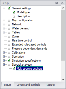
Figure: Accessing the multi-species analysis

Multi-species analysis editor¶

The editor allows to enter the input data by typing them into the text box. It also allows to load and export these data from/to a .msx file with the multi-species definitions.

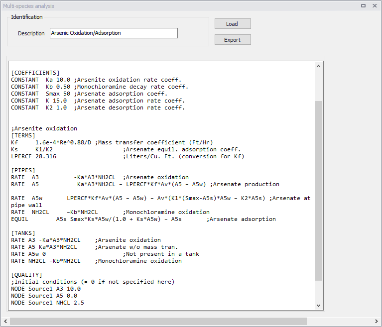
Figure: The Multi-species analysis editor

The following attributes are available:

Description: An optional description of the species being described.
Text box: Input data for the muti-species simulation must be inserted in the wide text box. The format matches the format of the .msx file used by the EPANT MSX engine. This format is described in more details in the section 'Multi-species definition format'.
Load: Load/import the multi-species definition from a .msx file.
Export: Save the multi-species definition into a .msx file. This is optional, and not required prior to running the simulation.

Multi-species definition format¶

The text box in the 'Multi-species analysis' editor can contain the following sections.

Section	Description
[TITLE]	adds a descriptive title to the data set
[OPTIONS]	sets the values of computational options
[SPECIES]	names the chemical species being analyzed
[COEFFICIENTS]	names the parameters and constants used in chemical rate and equilibrium expressions
[TERMS]	defines intermediate / auxiliary terms used in chemical rate and equilibrium expressions
[PIPES]	supplies the rates and equilibrium expressions that govern species dynamics in pipes
[TANKS]	supplies the rates and equilibrium expressions that govern species dynamics in storage tanks
[SOURCES]	identifies input sources (i.e., boundary conditions) for selected species supplies
[QUALITY]	supplies initial conditions for selected species throughout the network
[PARAMETERS]	allows parameter values to be assigned on a pipe-by-pipe basis
[PATTERNS]	defines time patterns used with input sources
[REPORT]	specifies reporting options

Table: Sections in Multi-species analysis editor

Below is an example content. Reserved keywords are shown in bold and option choices are separated by slashes.

[TITLE]
<title line>

[OPTIONS]
AREA_UNITS FT2/M2/CM2
TIME_UNITS SEC/MIN/HR/DAY
SOLVER EUL/RK5/ROS2
COUPLING FULL/NONE
TIMESTEP <seconds>
ATOL <value>
RTOL <value>

[SPECIES]
BULK <specieID> <units> (<atol> <rtol>)
WALL <specieID> <units> (<atol> <rtol>)

[COEFFICIENTS]
PARAMETER <paramID> <value>
CONSTANT <constID> <value>

[TERMS]
<termID> <expression>

[PIPES] or [TANKS]
EQUIL <specieID> <expression>
RATE <specieID> <expression>
FORMULA <specieID> <expression>

[SOURCES]
<type> <nodeID> <specieID> <strength> (<patternID>)

[QUALITY]
GLOBAL <specieID> <value>
NODE <nodeID> <bulkSpecieID> <value>
LINK <linkID> <bulkSpecieID> <value>

[PARAMETERS]
PIPE <pipeID> <paramID> <value>
TANK <tankID> <paramID> <value>

[REPORT]
NODES ALL
NODES <node1ID> <node2ID> …
LINKS ALL
LINKS <link1ID> <LINK2ID> …
SPECIES <species1ID> YES/NO (<precision>)
FILE <filename>
PAGESIZE <lines>

Data sections are described below. For more information about the multi-species analysis, visit https://www.epa.gov/water-research/epanet.

[TITLE]¶

Purpose: Provides a descriptive title to the problem being analyzed.

Format: A single line of text.

Remarks: The [TITLE] section is optional. In MIKE+, a default title made of the simulation ID and simulation description is used.

[OPTIONS]¶

Purpose: Defines various simulation options.

Formats:

AREA_UNITS: FT2/M2/CM2
TIME_UNITS: SEC/MIN/HR/DAY
SOLVER: EUL/RK5/ROS2
COUPLING: FULL/NONE
COMPILER: NONE/VC/GC
TIMESTEP: seconds
ATOL: value
RTOL: value

Definitions:

AREA_UNITS sets the units used to express pipe wall surface area where:
- FT2 = square feet (default)
- M2 = square meters
- CM2 = square centimeters
TIME_UNITS is the units in which all reaction rate terms are expressed. The default units are hours (HR).
SOLVER is the choice of numerical integration method used to solve the reaction system where:
- EUL = standard Euler integrator (default)
- RK5 = Runge-Kutta 5th order integrator
- ROS2 = 2nd order Rosenbrock integrator.
COUPLING determines to what degree the solution of any algebraic equilibrium equations is coupled to the integration of the reaction rate equations. If coupling is NONE, then the solution to the algebraic equations is only updated at the end of each integration time step. With FULL coupling the updating is done whenever a new set of values for the rate-dependent variables in the reaction rate expressions is computed. This can occur at several intermediate times during the normal integration time step when using the RK5 and ROS2 integration methods. Thus, the FULL coupling option is more accurate, but can require significantly more computation time. The default is NONE.
COMPILER determines if the chemical reaction system being modeled should first be compiled before the simulation begins. This option is available on Windows systems that have either the Microsoft Visual C++ or the MinGW compiler installed or on Linux systems with the Gnu C++ compiler. The VC option is used for the Visual C++ compiler, the GC option is for the MinGW or Gnu compilers, while NONE is the default which means that no compilation is performed. Using this option can result in faster run times by a factor of 2 to 5.
TIMESTEP is the time step, in seconds, used to integrate the reaction system. The default time step is 300 seconds (5 minutes).
ATOL is the default absolute tolerance used to determine when two concentration levels of a species are the same. It applies to all species included in the model. Different values for individual species can be set in the [[SPECIES]] section of the input (see below). If no ATOL option is specified, then it defaults to 0.01 (regardless of species concentration units).
RTOL is a default relative accuracy level on a species' concentration used to adjust time steps in the RK5 and ROS2 integration methods. It applies to all species included in the model. Different values for individual species can be set in the [[SPECIES]] section of the input (see below). If no RTOL option is specified, then it defaults to 0.001.

[SPECIES]¶

Purpose: Defines each chemical species being simulated.

Formats:

BULK: name units (Atol Rtol)
WALL: name units (Atol Rtol)

Definitions:

name: species name
units: species mass units
Atol: optional absolute tolerance that overrides the global value set in the [OPTIONS] section
Rtol: optional relative tolerance that overrides the global value set in the [OPTIONS] section

Remarks:

The first format is used to define a bulk water (i.e. dissolved) species while the second is used for species attached (i.e. adsorbed) to the pipe wall.
Bulk species are measured in concentration units of mass units per liter while wall species are measured in mass units per unit area.
Any units can be used to represent species mass. The user is responsible for including any necessary unit conversion factors when specifying chemical reaction and equilibrium expressions that involve several species with different mass units.
Values for both Atol and Rtol must be provided to override the default tolerances.

Examples:

[SPECIES]

;Bulk chlorine in mg/L with default tolerances

BULK CL2 MG

;Bulk biomass in ug/L with specific tolerances

BULK Xb UG 0.0001 0.01

;Attached biomass in ug/area with specific tolerances WALL Xa UG 0.0001 0.01

[COEFFICIENTS]¶

Purpose: Defines parameters and constants that are used in the reaction/equilibrium chemistry model.

Formats:

PARAMETER: name value
CONSTANT: name value

Definitions:

name: coefficient's identifying name
value: global value of the coefficient.

Remarks:

A PARAMETER is a coefficient whose value can be changed on a pipe-by-pipe (or tank-by-tank) basis (see the [[PARAMETERS]] section below) while a CONSTANT coefficient maintains the same value throughout the pipe network.

Examples:

[COEFFICIENTS]

;Kb can vary by pipe PARAMETER Kb 0.1 

;Kw is fixed for all pipes CONSTANT Kw 1.5

[TERMS]¶

Purpose: Defines mathematical expressions that are used as intermediate terms in the expressions for the chemical reaction/equilibrium model.

Formats: termID expression

Definitions:

termID: identifying name given to the term
expression: any well-formed mathematical expression involving species, parameters, constants, hydraulic variables or other terms.

Remarks:

Terms can be used to simplify reaction rate or equilibrium expressions that would otherwise be unwieldy to write all on one line or have the same terms repeated in several different rate/equilibrium equations. The definition and use of TERMS, when those terms are common and appear in multiple rate or equilibrium expressions, may speed computation because the common term expression requires only one evaluation.

Hydraulic variables consist of the following reserved names:

D: pipe diameter (feet or meters):
Q: pipe flow rate (flow units)
U: pipe flow velocity (ft/sec or m/sec)
Re: flow Reynolds number
Us: pipe shear velocity (ft/sec or m/sec)
Ff: Darcy-Weisbach friction factor
Av: Surface area per unit volume (area units/L)

Examples:

[TERMS]  
;A mass transfer coefficient  
Kf 1.2e-4*Re^0.88/D  
;A reaction term  
a1  k1*HOCL*NH3

[PIPES]¶

Purpose: Supplies the rate and equilibrium expressions that govern species dynamics in pipes.

Formats:

EQUIL: specieID expression
RATE: specieID expression
FORMULA: specieID expression

Definitions:

specieID: a species identifier
expression: any well-formed mathematical expression involving species, parameters, constants, hydraulic variables or terms.

Remarks:

There should be one expression supplied for each species defined in the model.
The allowable hydraulic variables are defined above in the description of the [[TERMS]] section.
The EQUIL format is used for equilibrium expressions where it is assumed that the expression supplied is being equated to zero. Thus, formally there is no need to supply the name of a species, but using one can help ensuring that all species are accounted for.
The RATE format is used to supply the equation that expresses the rate of change of the given species with respect to time as a function of the other species in the model.
The FORMULA format is used when the concentration of the named species is a simple function of the remaining species.

Examples:

[PIPES]  
;Bulk chlorine decay  
RATE CL2 -Kb*CL2 

;Adsorption equilibrium between Cb in bulk and Cw on wall EQUIL Cw Cmax*k*Cb / (1 + k*Cb) - Cw 

;Conversion between biomass (X) and cell numbers (N)  
FORMULA N log10(X*1.0e6) 

;Bulk C formation plus non-equilibrium sorption between C and Cs  
;Using hydraulic variable Av [Area-Units/Liter]  
RATE C K*C - Av*(K1*(Smax-Cs)*C - K2*Cs)  
;Equivalent sorption model, using 1/hydraulic radius = 4/D ;Assumes area units are FT2 and diameter in FT  
;CFPL is TERM equal to FT3/Liter, thus (4*CFPL/D) == Av  
RATE C K*C - (4*CFPL/D)*(K1*(Smax-Cs)*C - K2*Cs)

[TANKS]¶

Purpose: Supplies the rate and equilibrium expressions that govern species dynamics in storage tanks.

Formats:

EQUIL: specieID expression
RATE: specieID expression
FORMULA: specieID expression

Definitions:

specieID: a species identifier
expression: any well-formed mathematical expression involving species, parameters, constants, or terms.

Remarks:

A [TANKS] section is always required when a model contains both bulk and wall species, even when there are no tanks in the pipe network. If the model contains only bulk species, then this section can be omitted if the reaction expressions within tanks are the same as within pipes.
There should be one expression supplied for each bulk species defined in the model. By definition, wall species do not exist within tanks.
Hydraulic variables are associated only with pipes and cannot appear in tank expressions.
The EQUIL format is used for equilibrium expressions where it is assumed that the expression supplied is being equated to zero. Thus, formally there is no need to supply the name of a species but doing so helps ensuring that all species are accounted for.
The RATE format is used to supply the equation that expresses the rate of change of the given species with respect to time as a function of the other species in the model.
The FORMULA format is used when the concentration of the named species is a simple function of the remaining species.

Examples:

See the examples listed for the [PIPES] section.

[SOURCES]¶

Purpose: Defines the locations where external sources of particular species enter the pipe network.

Formats: sourceType nodeID specieID strength (patternID)

Definitions:

sourceType: either MASS, CONCEN, FLOWPACED, or SETPOINT
nodeID: the ID label of the network node where the source is located
specieID: a bulk species identifier
strength: the baseline mass inflow rate (mass/minute) for MASS sources or concentration (mass/L) for all other source types
patternID: the name of an optional time pattern that is used to vary the source strength over time.

Remarks:

Use one line for each species that has non-zero source strength.
Only bulk species can enter the pipe network, not wall species.
The definitions of the different source types conform to those used in the original EPANET program:
- A MASS type source adds a specific mass of species per unit of time to the total flow entering the source node from all connecting pipes.
- A CONCEN type source sets the concentration of the species in any external source inflow (i.e., a negative demand) entering the node. The external inflow must be established as part of the hydraulic specification of the network model.
- A FLOWPACED type source adds a specific concentration to the concentration that results when all inflows to the source node from its connecting pipes are mixed together.
- A SETPOINT type source fixes the concentration leaving the source node to a specific level as long as the mixture concentration of flows from all connecting pipes entering the node is less than the set point concentration.

If a time pattern is supplied for the source, it must be one defined in the [[PATTERNS]] section of the multi-species analysis definition, not a pattern from the associated EPANET simulation.

Examples:

[SOURCES]  
;Inject 6.5 mg/minute of chemical X into Node N1  
;over the period of time defined by pattern PAT1  
MASS N1 X 6.5 PAT1  
;Maintain a 1.0 mg/L level of chlorine at node N100  
SETPOINT N100 CL2 1.0

[QUALITY]¶

Purpose: Specifies the initial concentrations of species throughout the pipe network.

Formats:

GLOBAL: specieID concen
NODE: nodeID specieID concen
LINK: linkID specieID concen

Definitions:

specieID: a species identifier
nodeID: a network node ID label
linkID: a network link ID label
concen: a species concentration

Remarks:

Use as many lines as necessary to define a network's initial condition.
Use the GLOBAL format to set the same initial concentration at all nodes (for bulk species) or within all pipes (for wall species).
Use the NODE format to set an initial concentration of a bulk species at a particular node.
Use the LINK format to set an initial concentration of a wall species within a particular pipe.
The initial concentration of a bulk species within a pipe is assumed equal to the initial concentration at the downstream node of the pipe.
All initial concentrations are assumed to be zero unless otherwise specified in this section.
Models with equilibrium equations will require that reasonable initial conditions be set so that the equations are solvable. For example, if they contain a ratio of species concentrations then a divide by zero condition will occur if all initial concentrations are set to zero.

Examples:

[QUALITY]  
;Set concentration of bulk species Cb to 1.0 at all nodes GLOBAL Cb 1.0  
;Override above condition for node N100  
NODE N100 Cb 0.5

[PARAMETERS]¶

Purpose: Defines values for specific reaction rate parameters on a pipe-by-pipe or tank-by-tank basis.

Formats:

PIPE: pipeID paramID value
TANK: tankID paramID value

Definitions:

pipeID: the ID label of a pipe link in the network
tankID: the ID label of a tank node in the network
paramID: the name of one of the reaction rate parameters listed in the [COEFFICIENTS] section
value: the parameter's value used for the specified pipe or tank.

Remarks: Use one line for each pipe or tank whose parameter value is different than the global value.

[PATTERNS]¶

Purpose: Defines time patterns used to vary external source strength over time.

Formats: name multiplier multiplier ...

Definitions:

name: an identifier assigned to the time pattern
multiplier: a multiplier used to adjust a baseline value

Remarks:

Use one or more lines for each time pattern included in the model.
If extending the list of multipliers to another line remember to begin the line with the pattern name.
All patterns share the same time period interval as defined in the [TIMES] section of the EPANET input file being used in conjunction with the EPANET-MSX input file.
Each pattern can have a different number of time periods.
When the simulation time exceeds the pattern length the pattern wraps around to its first period.

Examples:

[PATTERNS]  
;A 3-hour injection pattern over a 24-hour period ;(assuming a 1-hour pattern time interval is in use) 

P1 0.0 0.0 0.0 0.0 1.0 1.0  
P1 1.0 0.0 0.0 0.0 0.0 0.0  
P1 0.0 0.0 0.0 0.0 0.0 0.0  
P1 0.0 0.0 0.0 0.0 0.0 0.0

[REPORT]¶

Purpose: Describes the content of the output report produced from a simulation.

Formats:

NODES: ALL
NODES: node1, node2, etc.
LINKS: ALL
LINKS: link1, link2, etc.
SPECIES: speciesID YES/NO (precision)
FILE: filename
PAGESIZE: lines

Definitions:

node1,node2, etc.: a list of nodes whose results are to be reported
link1,link2, etc.: a list of links whose results are to be reported
specieID: the name of a species to be reported on
precision: number of decimal places used to report a species' concentration
filename: the name of a file to which the report will be written
lines: the number of lines per page to use in the report.

Remarks:

Use as many NODES and LINKS lines as it takes to specify which locations get reported. The default is not to report results for any nodes or links.
Use the SPECIES line to specify which species get reported and at what precision. The default is to report all species at two decimal places of precision.
The FILE line is used to have the report written to a specific file. If not provided the report will be written to the same file used for reporting program errors and simulation status.

Examples:

[REPORT\ 
;Write results for all species at all nodes and links  
;at all time periods to a specific file  
NODES ALL  
LINKS ALL

Running analysis¶

In order to run the multi-species simulation, open the Simulation setup editor and select the 'Multi-species water quality' module. When this module is selected, two simulation modes are available: you can either run both hydraulics and water quality simulations at the same time, or you can run only the water quality simulation using an "hydraulics" file resulting from an earlier hydraulics simulation. The latter helps reducing simulation times when the hydraulic simulation takes a long time and does not need to be repeated while running the water quality scenarios. The input hydraulics file is saved from the hydraulics simulation by selecting 'Save hydraulics file' in the 'Output' tab.

The simulation reports error and warning messages into the .sum file. Some of the simulation errors that result in the program termination are described below:

Error 513: could not integrate reaction rate expressions. The differential equation solver employed by EPANET MSX could not successfully integrate the system's reaction rate equations over the current water quality time step. One could try re-running the analysis using a smaller time step or larger values for ATOL and RTOL (as specified in the [OPTIONS] or [SPECIES] sections of the multi-species analysis definition).
Error 514: could not solve reaction equilibrium expressions. The non-linear equation solver employed by EPANET MSX could not successfully solve the system's set of equilibrium equations at the current simulation time. Users must ensure that the initial conditions set throughout the pipe network are sufficient and consistent so that a solution exists for the governing set of equilibrium equations.

In case that the multi-species simulation is unable to find the solution, adjustments to the model setup might be necessary such as:

Use smaller time step or large values for tolerance parameters
Change the solver type (numerical integration method)
Change the coupling type
Reduce the size and complexity of the model network by removing short dead-end pipes and merging pipes together in order to reduce number of pipes and to remove short pipe segments.

Simulation results¶

The simulation results are stored in the .msxr results file, and they can be processed in the same way as any other results.

Examples of multi-species analysis definition¶

Several examples of multi-species analysis definitions are provided in this section. They can be applied to any hydraulic model with only few or minor modifications, such as change of the tank ID's, for example. For more information about the multi-species analysis and sample MSX files, visit: https://www.epa.gov/water-research/epanet.

Two-source chlorine decay¶

Multi-source networks present problems when modelling a single species, such as free chlorine, when the decay rates observed in the source waters vary quite significantly. As the sources blend differently throughout the network it becomes difficult to assign a single decay coefficient that accurately reflects the decay rate observed in the blended water. One approach to reconciling the vastly different chlorine decay constants in this example, without introducing a more complex chlorine decay mechanism that attempts to represent the different reactivity of the total organics from the two sources, is to assume that at any time the chlorine decay constant within a pipe is given by a weighted average of the two source values, where the weights are the fraction of each source water present in the pipe. These fractions can be deduced by introducing a fictitious conservative tracer compound at Source 1, denoted as T1, whose concentration is fixed at a constant 1.0 mg/L. Then at any point in the network the fraction of water from Source 1 would be the concentration of T1 while the fraction from Source 2 would be 1.0 minus that value. The resulting chlorine decay model now consists of two-species, a tracer species T1 and a free chlorine species C.

[OPTIONS]  
AREA_UNITS  FT2  
RATE_UNITS  HR  
SOLVER      RK5  
TIMESTEP    300

[SPECIES]  
BULK T1 MG ;Source 1 tracer  
BULK CL2 MG ;Free chlorine

[COEFFICIENTS]  
CONSTANT k1 1.3 ;Source 1 decay coeff.
CONSTANT k2 17.7 ;Source 2 decay coeff.

[PIPES]  
;T1 is conservative  
RATE T1 0  
;CL2 has first order decay  
RATE CL2 -(k1*T1 + k2*(1-T1))*CL2

[QUALITY]  
;Initial conditions (= 0 if not specified here)  
[QUALITY]  
;Initial conditions (= 0 if not specified here)  
NODE Source1 T1 1.0  
NODE Source1 CL2 1.2  
NODE Source2 CL2 1.2

[REPORT]  
NODES ALL  
LINKS ALL

Mass transfer-limited arsenic oxidation/adsorption system¶

This example is an extension and more complete description of the arsenic oxidation/adsorption model. It models the oxidation of arsenite As+3 to arsenate As+5 by a monochloramine disinfectant residual NH2Cl in the bulk flow along with the subsequent adsorption of arsenate onto exposed iron on the pipe wall. We also include a mass transfer limitation to the rate at which arsenate can migrate to the pipe wall where it is adsorbed. It assumes that the network has a single source which is a reservoir node Source1.

[SPECIES]  
BULK A3 UG ;Dissolved arsenite  
BULK A5 UG ;Dissolved arsenate  
BULK A5w UG ;Dissolved arsenate at wall  
WALL A5s UG ;Adsorbed arsenate  
BULK NH2CL MG ;Monochloramine 

[COEFFICIENTS]  
CONSTANT  Ka 10.0 ;Arsenite oxidation rate coeff.  
CONSTANT  Kb 0.50 ;Monochloramine decay rate coeff.  
CONSTANT  Smax 50 ;Arsenate adsorption coeff.  
CONSTANT  K 15.0  ;Arsenate adsorption rate coeff.  
CONSTANT  K2 1.0  ;Arsenate desorption rate coeff. 

;Arsenite oxidation  
[TERMS]  
Kf 1.6e-4*Re^0.88/D;Mass transfer coefficient (Ft/Hr) 
Ks K1/K2;Arsenate equil. adsorption coeff.
LPERCF 28.316;Liters/Cu. Ft. (conversion for Kf)

[PIPES]  
RATE A3 -Ka*A3*NH2CL;Arsenate oxidation
RATE A5 Ka*A3*NH2CL - LPERCF*Kf*Av*(A5 - A5w);Arseate production

RATE A5wLPERCF*Kf*Av*(A5 - A5w) - Av*(K1*(Smax-A5s)*A5w - K2*A5s) ;Arsenate at pipe wall 
RATE NH2CL-Kb*NH2CL ;Monochloramine oxidation  
EQUIL A5s Smax*Ks*A5w/(1.0 + Ks*A5w) - A5s ;Arsenate adsorption

[TANKS]  
RATE A3 -Ka*A3*NH2CL;Arsenite oxidation
RATE A5 Ka*A3*NH2CL;Arsenate w/o mass tran.
RATE A5w 0;Not present in a tank
RATE NH2CL -Kb*NH2CL ;Monochloramine oxidation

[QUALITY]  
;Initial conditions (= 0 if not specified here)  
NODE Source1 A3 10.0  
NODE Source1 A5 0.0  
NODE Source1 NHCL 2.5

[REPORT]  
NODES ALL  
LINKS ALL

Bacterial regrowth model with chlorine inhibition¶

This example models bacterial regrowth as affected by chlorine inhibition within a distribution system. There are six species defined for the model: bulk chlorine (CL2), bulk biodegradable dissolved organic carbon (S), bulk bacterial concentration (Xb), bulk bacterial cell count (Nb), attached bacterial concentration (Xa), and attached bacterial cell count (Na). CL2 and S are measured in milligrams. The bacterial concentrations are expressed in micrograms of equivalent carbon so that their numerical values scale more evenly. The bacterial cell counts are expressed as the logarithm of the number of cells. The model assumes that there is a single source node named Source1 that supplies all water to the system.

[OPTIONS]  
AREA_UNITS CM2
RATE_UNITS HR
SOLVER RK5
TIMESTEP 300

[SPECIES]  
BULK CL2 MG ;chlorine  
BULK S MG    ;organic substrate  
BULK Xb UG    ; mass of free bacteria  
WALL Xa UG    ; mass of attached bacteria  
BULK Nb log(N) ;number of free bacteria  
WALL Na log(N) ;number of attached bacteria

[COEFFICIENTS]  
CONSTANT Kb 0.05 ;CL2 decay constant (1/hr)
CONSTANT CL2C 0.20 ;characteristic CL2 (mg/L)
CONSTANT CL2Tb 0.03 ;threshold CL2 for Xb (mg/L)
CONSTANT CL2Ta 0.10 ;threshold CL2 for Xa (mg/L)
CONSTANT MUMAXb 0.20 ;max. growth rate for Xb (1/hr)
CONSTANT MUMAXa 0.20 ;max. growth rate for Xa (1/hr)
CONSTANT Ks 0.40 ;half saturation constant (mg/L)
CONSTANT Kdet 0.03 ;detachment rate constant (1/hr/(ft/s))
CONSTANT Kdep 0.08 ;deposition rate constant (1/hr)
CONSTANT Kd 0.06 ;bacterial decay constant (1/hr)
CONSTANT Yg 0.15 ;bacterial yield coefficient (mg/mg)

[TERMS]  
Ib EXP(-STEP(CL2-CL2Tb)*(CL2-CL2Tb)/CL2C) ;Xb inhibition coeff.  
Ia EXP(-STEP(CL2-CL2Ta)*(CL2-CL2Ta)/CL2C) ;Xa inhibition coeff.  
MUb MUMAXb*S/(S+Ks)*Ib ;Xb growth rate coeff.
MUa MUMAXa*S/(S+Ks)*Ia ;Xa growth rate coeff.

[PIPES]  
RATE CL2 -Kb*CL2
RATE S -(MUa*Xa*Av + MUb*Xb)/Yg/1000
RATE Xb (MUb-Kd)*Xb + Kdet*Xa*U*Av - Kdep*Xb
RATE Xa (MUa-Kd)*Xa - Kdet*Xa*U + Kdep*Xb/Av
FORMULA Nb LOG10(1.0e6*Xb)
FORMULA Na LOG10(1.0e6*Xa)

[TANKS]  
RATE CL2 -Kb*CL2
RATE S -MUb*Xb/Yg/1000
RATE Xb (MUb-Kd)*Xb
FORMULA Nb LOG10(1.0e6*Xb)

[SOURCES]  
CONCEN Source1 CL2 1.2
CONCEN Source1 S 0.4
CONCEN Source1 Xb 0.01

[REPORT]  
NODES ALL  
LINKS ALL