Profile Plots
Profile plots can be created from the main Map view, with or without results, or from a map result plot.
A profile plot is drawn between specified flags. If there are two or more possible paths between two flags, the path with the smallest number of links (smallest number of pipes, or smallest number of river reaches delimited by connections to other rivers or pipes) will be selected. Hence, in order to better control the path, more flags should be set until a unique path between flags can be identified. If multiple pipes exist between the same two nodes, the active pipe with the largest diameter or height will be selected.
The selected path can be seen on the map using the 'Connect flags' option. Using this option is however optional, and it is possible to draw the profile plot without connecting the flags.
Creating Profile Plots from the Map
Profile plots can be created from the model map (i.e. Map View) with or without simulation results.
- On the Map View, define path flags via ‘Set flags’ on the ‘Profile and Tracing’ toolbox on the Map ribbon (figure below).
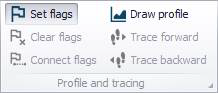
Figure: The Profile and Tracing toolbox on the Map ribbon
- Click on the starting location for the profile path. Flags can be set on nodes, junctions, and rivers. This will place a small flag at the selected location along with the number of the flag.
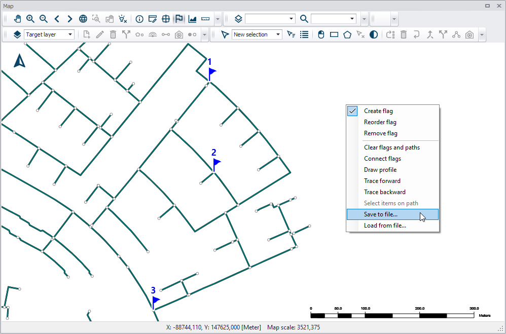
Figure: Set flags defining the path of the profile plot on the model map
- Continue setting flags on the map until the path is well-defined. The horizontal plan will then look as seen in the figure above. You may save the set flag information using the ‘Save to file...’ option from the local context menu. The path information is saved to a *.path file, which can be loaded in another session via the 'Load from file...' option.
- Finally, click on ‘Draw profile’ on the Profile and Tracing toolbox. This will create a new profile plot (figure below).
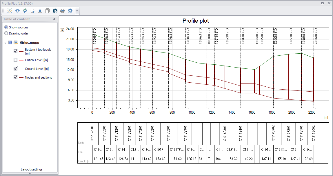
Figure: The Profile Plot form window showing an example longitudinal profile plot without simulation results
Profile Plot with Results
When result files are available, default results are plotted when a profile plot is created. Result items can also be added to a profile plot, following these steps.
- From a profile plot, use the 'Add item' button from the upper toolbar or from the local context menu (i.e. right-click) in the left panel (figure below). Alternatively, drag a result item (e.g. Link Water Level) from the list of result files in the 'Results' tree, and drop it in the table of content of the profile plot.
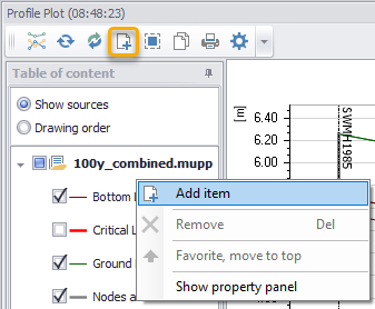
Figure: The ‘Add item’ tool on the Profile Plot window
- Specify the result file, item, and data type to add to the profile plot on the ‘Add item’ dialog that appears (figure below).
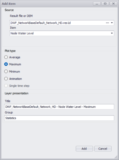
Figure: The ‘Add item’ dialog where the result file and items to add to the profile plot are defined
- If the selected result file is a 'LTS extreme statistics' type of file, the plot type is always a single time step representing a recurrence interval, which must be selected from the list which appears in the 'Add item' dialog. The left list contains computed recurrence intervals saved in the result file, whereas the right list allows specifying custom recurrence intervals for which the results are interpolated using a linear interpolation method from the recurrence intervals in the result file.
- If the selected result file is a 2D file from a 2D overland simulation, a maximum spacing must also be specified: it controls the spacing between points along the 2D profile.
The added result item then appears on the Profile Plot (figure below). Result items are plotted on the secondary (i.e. right) y-axis, when their item type differs from an elevation.
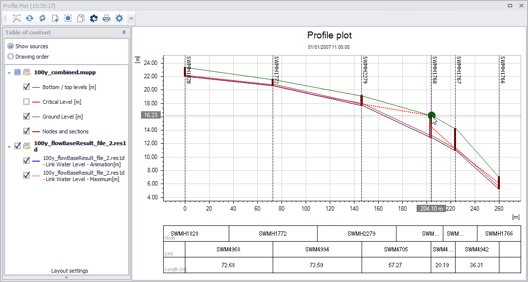
Figure: The Profile Plot form window showing an example longitudinal profile plot with max. link water level simulation results (red broken line)
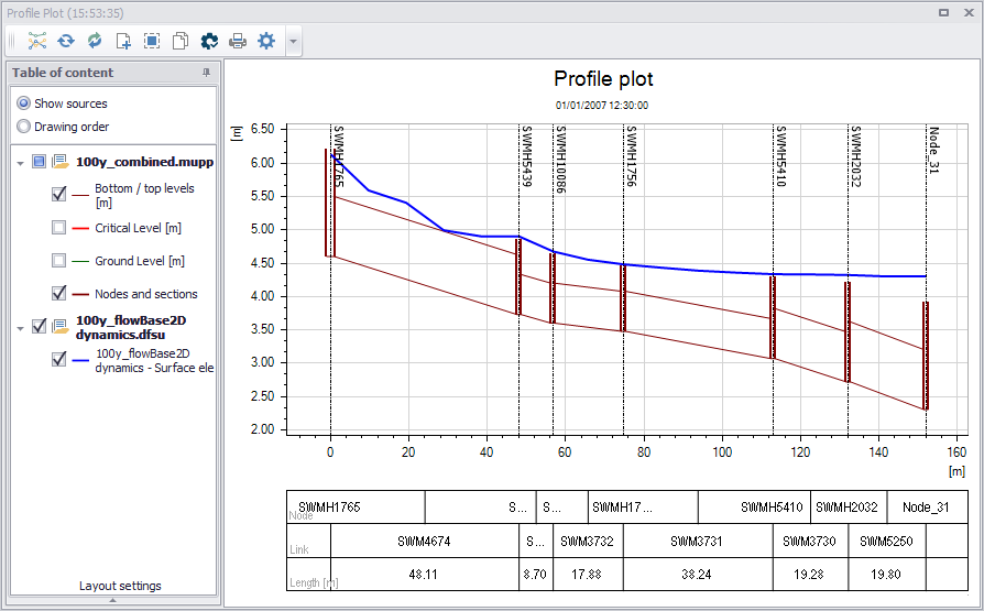
Figure: The Profile Plot form window showing an example longitudinal profile plot 2D water level simulation results (blue line)
When result items are added to the profile plot, it is possible to change the presentation mode (choice between Animation, Maximum, Minimum or Average type) afterwards. This option is offered from the local context menu, with a right-click on the related result item.
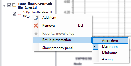
Figure: The selection of result presentation mode for a result item
Profile Plot with DEM
DEM profiles can also be added to a profile plot. DEM profiles can be obtained either from raster files or from 2D flexible mesh files, following these steps:
- From a profile plot window, use the 'Add item' button or the 'Add item' option in the local context menu (i.e. right-click) on the left panel.
Figure: The 'Add item' tool on the Profile Plot window
- Select the DEM file, as well as the item if the file contains multiple items. A maximum spacing must also be specified: it controls the spacing between points along the DEM profile (figure below).
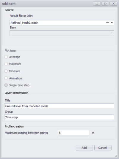
Figure: The 'Add item' dialog where the DEM file and settings are specified
The DEM item then appears on the Profile Plot (figure below). Result items are plotted on the secondary (i.e. right) y-axis.
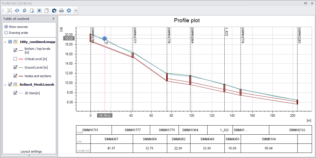
Figure: The Profile Plot form window showing an example longitudinal profile plot with a DEM profile (blue broken line)
The DEM profile is plotted with one point at each node's location, plus additional points in-between in order to fulfill the specified maximum spacing.
When a 2D overland model is defined, a default DEM profile is added to new profile plots, using the 2D domain as source of DEM.
Creating Profile Plots from a Result Map
Profile plots may also be created from extra result maps (obtained from the ‘Create result map’ button). The profile tools that can be used with this type of maps are located on the Results menu ribbon.
- First, create a result map plot as described in chapter Displaying Results on a Map.
- Set path flags on the result map using the ‘Set flags’ tool from the Profile Plot toolbox on the Results ribbon (figure below).
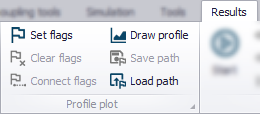
Figure: Set flags from the Profile Plot toolbox on the Results ribbon
- Click on the starting node for the profile path. This will place a small flag next to the node along with the number of the flag. Continue setting flags on the result map until the path is well-defined. Having both point (i.e. node) and line (i.e. link) result features on a result map helps with path-setting.
- Finally, click on ‘Draw profile’ on the Profile Plot toolbox. This will create a new profile plot on a profile plot form.
- Default items are added when creating the profile plot. Other result items may be added as described in the section Profile Plot with Results.
The Profile Plot Window
The Profile Plot window displays longitudinal profile plots created in the project. Its various parts and components are described in succeeding sections.
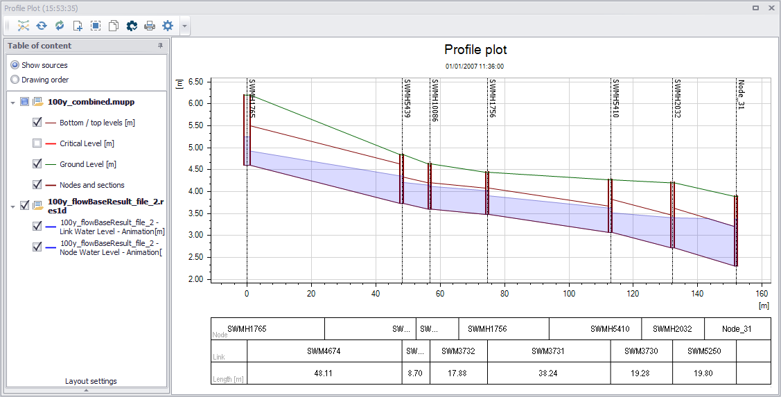
Figure: The Profile Plot window
Table of Content
The table of content (TOC) panel is located on the left side of the profile plot form. The panel lists information on the various information layers that are used for the profile plot.
At the top of the panel, it is possible to select between two different types of views in the TOC:
- Show sources: This option groups data layers according to data source and indicates the file from which the data are obtained.
- Drawing order: Use this option to allow reordering/grouping of data layers on the plot. Reorder or group layers by dragging layer labels up or down the TOC list.
When right-clicking on the panel, the local context menu opens up (see figure below), offering a number of options described below.
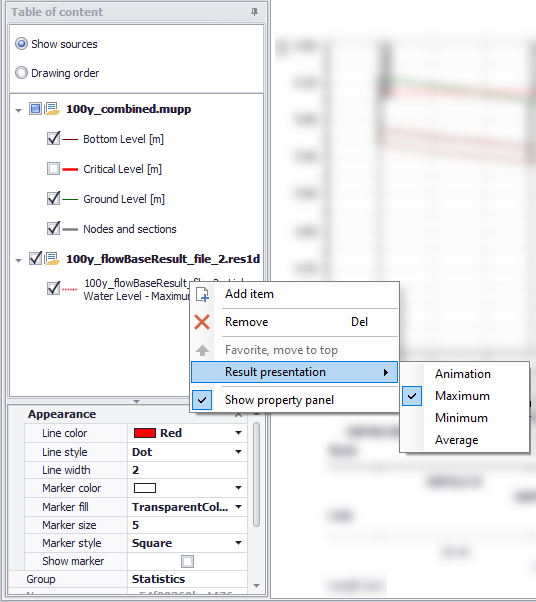
Figure: The local context menu on the longitudinal profile
Add item
Use this option to add result items or DEM items to an existing profile plot. See Profile Plot with Results and Profile Plot with DEM.
Remove
Use this option to remove a layer from the profile plot.
Result presentation
Use this option to select the presentation mode of a result item. Possible modes are Animation (showing instantaneous results for the current date and time), Maximum, Minimum or Average.
Show property panel
Activate this option to view the Property Panel below the TOC. The Property Panel is used to customize the appearance of data layers on the profile plot.
Alternatively, click on the expand arrow icon at the bottom of the TOC to view the Property Panel.
Property Panel
The Property Panel is used to customize the appearance of data layers on the profile plot.
Select a layer from the TOC to view its properties on the Property Panel. Customize layer properties on the panel as needed. See figure below.
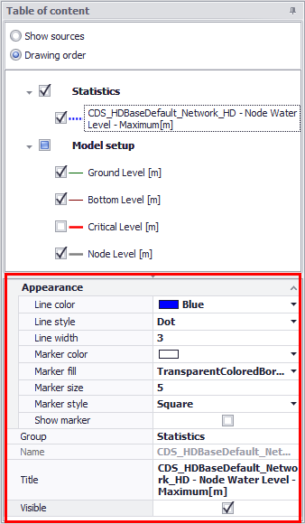
Figure: The Property Panel on the Profile Plot window
Plot Context Menu
Right-click on the profile plot to access the local context menu.
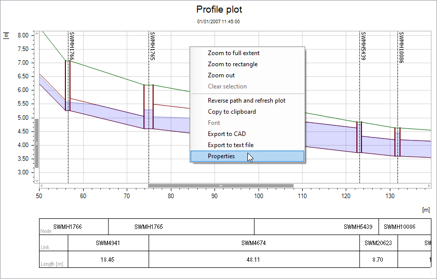
Figure: Right-click on the plot to access the local context menu
Zoom to full extent, Zoom to rectangle, Zoom out
Allows to zoom in and out on the plot. While zooming to a rectangle, dragging to draw a horizontal line will display arrows to zoom along the horizontal axis only, keeping the vertical axis unchanged. Similarly, dragging to draw a vertical line will zoom along the vertical axis only.
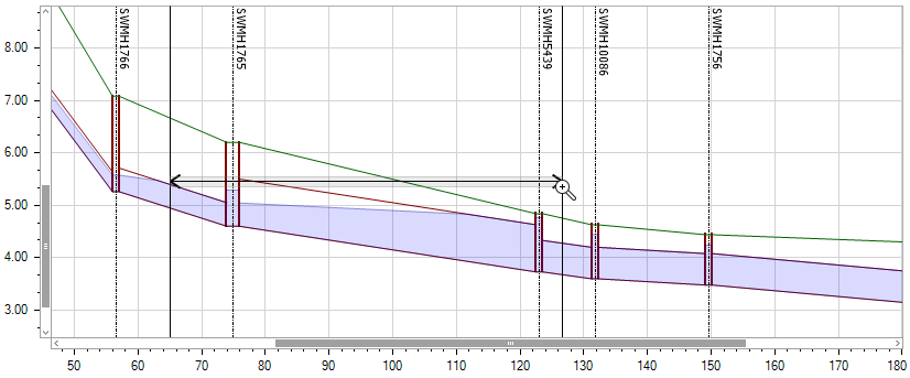
Figure: Use the ‘Zoom to rectangle’ option to zoom along one axis only
Zoom to full extent brings you back to the full view of visible data layers on the profile plot. Panning is also enabled upon activation of zoom options.
Note
Additional options are available to control the zoom options:
- Hold down the Shift key, to enable 'Zoom to rectangle'
- Scroll with the mouse wheel to zoom in or out.
Clear selection
Deselects selected elements in the longitudinal profile.
Reverse path and refresh plot
Will swap the profile, e.g. swap profile from being drawn from node A to node B (from left to right on the plot) to being drawn from node B to node A.
Copy to clipboard
Copies the longitudinal profile displayed to the clipboard and allows it to be pasted into other applications.
Export to CAD
Opens the ‘CAD export options’ window to export the profile plot view to a CAD file.
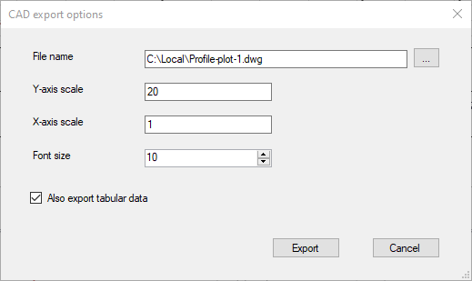
Figure: The ‘CAD export options’ window
From this window, it is possible to select a folder location as well as a file name for the created CAD file.
The X-axis and Y-axis scales control the lengths of the horizontal and vertical axes in the CAD file. They define scales relative to lengths in this CAD file.
The selected font size applies to all texts and values saved in the CAD file: select an appropriate font size that fits e.g. the exported axes and table.
Data in the table below the profile plot are exported to the CAD file only if ‘Also export tabular data’ option is selected.
Export to text file
Export the data from the profile plot view to a text file.
This text file contains a table with columns separated by semicolons. All data items (Link ID, Node ID, distance along the profile plot, elevations, etc.) are listed in columns, whereas the various links are listed in rows. When result items exist on the profile plot, they are also exported to extra columns in the file. The result value exported is the value shown on the plot (e.g. current time step for animated results, or maximum value, etc.).
Note for collection system networks
When exporting data from a collection system network with results, some of the links may contain multiple calculation points depending on their length. In this case, all calculation points' values are listed in the same cell with a separator, for example like this: 6.96499 6.87148 6.78332.
Note for river networks
When exporting river networks, each river is exported as a link but extra information is exported at each cross section location. The exported table will also contain information at "virtual node" locations, a virtual node being the location of a flag controlling the profile plot locations. Virtual nodes therefore do not represent actual calculation points on the network, and will show interpolated values.
Properties
Activate this option to view the Profile Plot Properties dialog.
Profile Plot Tools
The toolbar on top of the Profile Plot window offers several tools that may be used for working with profile plots.
New plot

Generate a new profile plot (on the existing profile plot window) from a new set of defined path flags.
Refresh

Update/refresh existing data layers on the plot. Ensures that changes to model data (e.g. node invert level via the Nodes editor) for elements included in the profile are reflected in the plot. The location of the profile plot is not changed even if flags have been moved on the map.
Reverse path and refresh plot

Swaps the left to right plot path orientation going from first to the last flag locations to last to first flag locations.
Add item

Use this option to add result items or DEM items to the profile plot. See Profile Plot with Results and Profile Plot with DEM. Result items presenting elevation results are plotted on the left y-axis, whereas other types of results are plotted on the right y-axis.
Selection mode

Allows for selecting model elements from the longitudinal profile. It uses ‘Select by rectangle’ option. Selected elements are also highlighted on the Map. The displayed selection in the profile is synchronized with both the map and the editors.
Copy to clipboard

Copies the longitudinal profile displayed to the clipboard and allows it to be pasted into other applications.
Set as default
![]()
Changes the default layout of the profile plot in the current MIKE+ project, to match the layout of the current profile plot. After pressing this button, the layout of the current profile plot will therefore apply to new plots, i.e. showing the same layers and with the same layer properties.
Print/Export

Option for formatting the plot for printing. Launches the print preview window. See section Print/Export Preview.
Properties

Launches the Profile Plot Properties dialog. See section Profile Plot Properties.
Save to plots manager
![]()
Saves the profile plot (path along the network, list of result items plotted and display settings) to the 'Plots' panel. The profile plot will initially be added to the active folder from this panel. See 'Plots Management' chapter (page 496) for more information on options to save and manage results windows.
Print/Export Preview
The Print/Export tool from the Profile Plot toolbar launches the Preview window, wherein print layouts for the plot may be configured.
It also allows for exporting the plot layout to various document file types for potential inclusion in reports or information dissemination.
File Menu
The File menu on the Preview window offers options for:
- Export Document. Export the layout to documents in the following format:
- HTML
- MHT
- RTF
- XLS
- XLSX
- Image File (e.g. PNG, JPG, etc.)
- Send via E-mail. Exports the layout to a document (as above) and then launches the email program including the document as attachment to an email for sending.
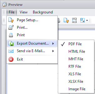
Figure: Preview window File menu
View Menu
The View menu offers options for modifying the appearance of the Preview window:
- Page Layout. Customize the layout display on the window. ‘Facing’ displays facing pages at once.
- Toolbar and Status Bar. Options for adding or removing the respective components from the window.
- Customize. Launches the Customization dialog, where various options for further modifying the window are available. These options include:
- Activating/deactivating toolbars
- Creating custom toolbars
- Enlarging toolbar icons
- Activating/deactivating tooltips
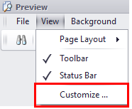
Figure: The View menu on the Preview window allows for customization of the window appearance and toolbars
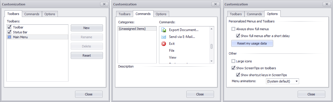
Figure: Various options for modifying the appearance of the Preview window on the Customization dialog
Background Menu
Customize the layout background via the Background menu. It offers options for:
- Color. Modifying the solid layout background color.
- Watermark. Launches the Watermark dialog, where text and/or image watermarks may be added to the layout.
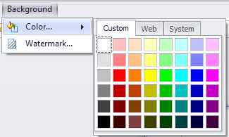
Figure: The Background menu on the Preview window
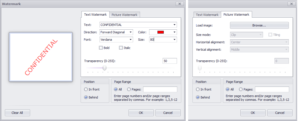
Figure: Add text or image watermarks to layouts via the Watermark dialog
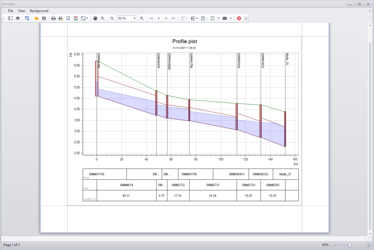
Figure: The Print/Export Preview window
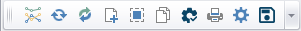
Preview Toolbar

The toolbar on the Preview window offers various tools for working with the layout.
Search

Text search on the plot.
Customize

Offers options for plot resizing during printing: None, Stretch, or Zoom.
Open

Option for loading an existing preview document *.PRNX layout configuration file.
Save

Option for saving the layout configuration in a preview document *.PRNX file.
Print

Launches the Print dialog where printing options may be customized before actual printing.
Quick Print

Option for immediate printing of layout using current configuration.
Page Setup

Launches the Page Setup dialog for defining layout printing setup.
Header and Footer

Launches the Header and Footer dialog, where custom page headers and footers may be defined.
Hand Tool

Tool for panning around the layout.
Magnifier, Zoom Out, Zoom In, Zoom

Tools for zooming in and out on the layout.
Color

Customize the layout background color.
Watermark

Launches the Watermark dialog for adding text and/or image watermarks to the layout.
Export Document

Exports the layout to a document.
Send via Email

Exports the layout to a document and adds it as attachment to a new email for sending.
Exit

Closes the Preview window.
Profile Plot Properties
Lower buttons
The properties of the longitudinal profile can be changed via the Properties dialog (figure below). The dialog is accessed in several ways:
- Choose ‘Properties’ on the local context menu on the profile plot area.
- Double-click on the profile plot area.
- Activate the Properties tool from the Profile Plot toolbar.
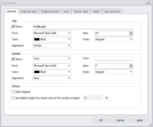
Figure: Setting the properties of the profile plot
The dialog has various tab pages wherein changes to the profile plot properties can be made. The following general button functionalities are available at the bottom of the dialog:
OK
Apply the settings specified and close the properties dialog.
Cancel
Cancel any changes made and close the properties dialog.
Apply
Apply the settings specified, but leave the properties dialog open.
General
The General tab page offers options for:
- Adding and formatting plot titles
- Adding and formatting subtitles
- Showing the data Legend
- Controlling the height of the table below the profile plot (height expressed as a percentage of the entire window's height)
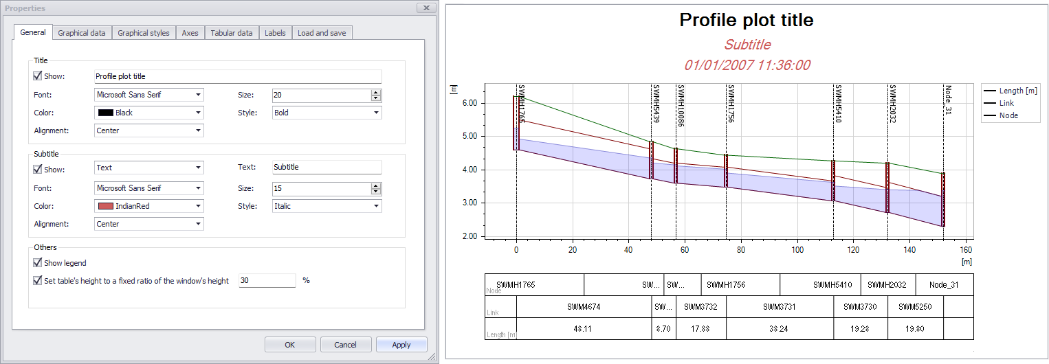
Figure: Customizing the plot title and subtitle via the General tab
Graphical Data
On the Graphical Data page, it is possible to specify which general information is to be shown on the profile plot. The various display options available for the graphical items can be reviewed and changed on this page.
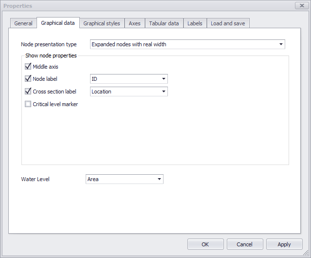
Figure: The Graphical Data tab
- Node presentation type: this controls the type of presentation for nodes along collection system networks (in 'Rivers, collection system and overland flows' mode only). The available options are:
- Collapsed nodes. To not show node lateral dimensions on the longitudinal profile. Useful for long profiles with many nodes.
- Expanded nodes with real width. To show node lateral dimensions the longitudinal profile, using the actual nodes’s width.
- Expanded nodes with fixed width. To show node lateral dimensions on the longitudinal profile, using a fixed width regardless of the actual node's size. Useful to keep showing node results, while keeping their size limited for showing long network path. With this mode, when a node symbolic width becomes larger than half of the connected link length (e.g. when zooming out), the node will automatically collapse in order to keep showing long network paths.
- Node label: Toggles on/off labels for nodes above the node in the profile. Select the label parameter from the dropdown menu on the right.
- Cross section label: Toggles on/off labels for cross sections in the profile. Select the label parameter from the dropdown menu on the right. This is only available for river networks in 'Rivers, collection system and overland flows' mode.
- Critical level: Toggles on/off display of critical levels within nodes on the longitudinal profile. This critical level markers are only displayed in the extent of the nodes, as opposed to the 'Critical level' layer available in the table of content of the profile, which displays a line interpolated between nodes. This is only available for collection system networks in 'Rivers, collection system and overland flows' mode.
- Water level: Option for showing either only the water surface line, or only the water level filling in the pipes, or both. Note: if both line and filling are selected, and if the profile plot includes both nodes and links water levels, the water surface line will only display the link water level line, in order to avoid overlapping lines.
Graphical Styles
Format profile plot data layer appearance on the Graphical Styles tab page. For each data item, line symbol style, width, and color may be customized. In addition, markers may be included, and marker appearance defined.
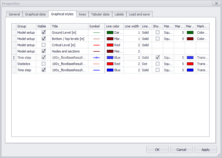
Figure: The Graphical Styles tab
Axes
The Axes tab page offers options for setting axes properties, including axes labels and grid lines. It has options for:
- Customizing axes title and label fonts
- Modifying axes line appearance
- Formatting the title, scale, label, grid lines, and visual range for the x-axis
- Formatting the title, scale, label, grid lines, and visual range for the primary (i.e. left) y-axis
- Formatting the title, scale, label, grid lines, and visual range for items on the secondary (i.e. right) y-axis. Result items are plotted on the secondary (i.e. right) y-axis.

Figure: The Axes tab page
Tabular Data
The Tabular Data tab page offers an option for configuring the content of the table below the profile plot.
From the 'Common data' tab, select the attributes to include in the table which are common to all link layers (e.g. pipes, rivers, valves, weirs, etc.) or node layers (typically nodes or junctions). From the 'Additional data' tab, select the extra attributes to show, specifically for each individual table of the database. To add an item to the profile plot window, tick its 'Show in table' box.
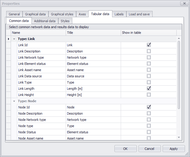
Figure: The Tabular Data tab is used to control the content of the table
The 'Styles' tab allows formatting the content of the table. It can especially be used to control the order of the displayed items (rows) in the table, customize their displayed names, control the font and its rotation, or adjust the heights of the rows.
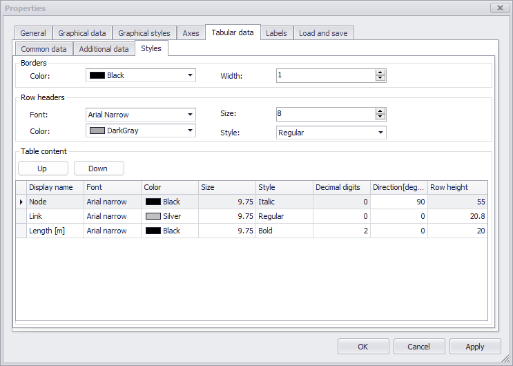
Figure: The Tabular Data tab allows customizing the styles of the table's data
Labels
Add custom text labels to the profile plot via the Labels tab page. ‘Add’ a new custom label and define it’s location and text annotation. Custom labels could be placed at locations relative to model object positions (e.g. nodes, links, etc.).
Save custom label configurations into profile plot label files via the ‘Save to file’ option. Existing label configurations may be loaded through ‘Load from file’.
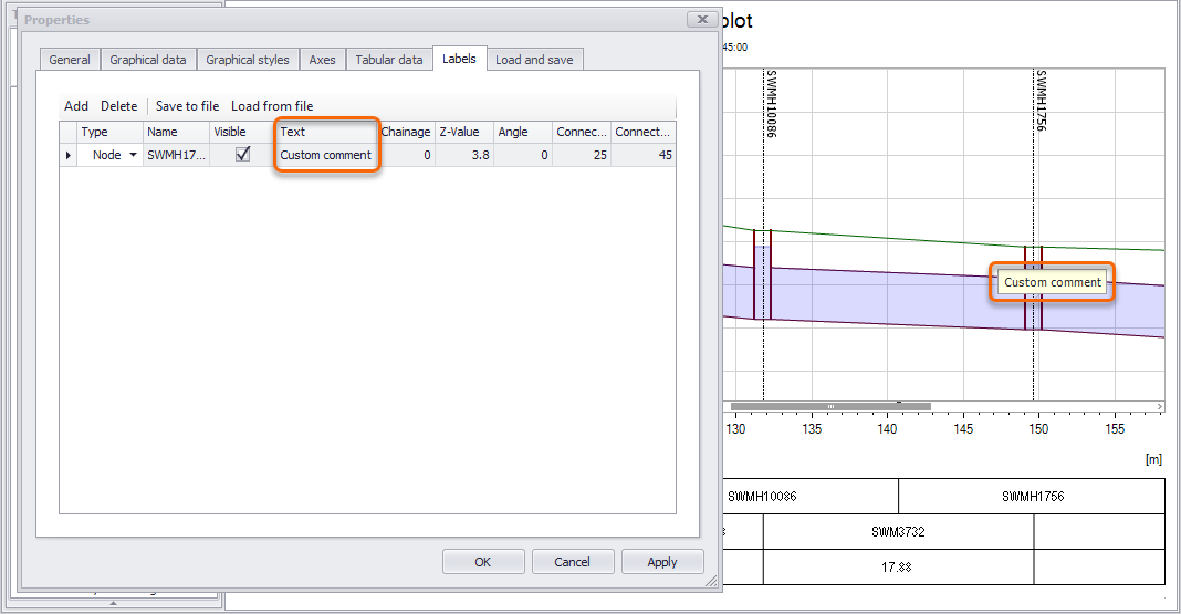
Figure: The Labels tab page showing an example custom label by a node
Load and Save
This tab contains options to re-use a custom layout and a path. The layout covers the list of layers shown on the profile plot (including result layers), their graphical styles, the axes style, the additional X-axis data, the plot's title, etc. The plot's path is defined by the location of the flags on the map, used to create the profile plot's path. This path is not saved in the layout definition.
The ‘Save to file’ option (in the ‘Layout’ group) saves the current profile’s layout to a profile plot file (*.profileplot) containing the layout definition.
The ‘Load from file’ option loads a profile layout file (*.profileplot) to update the current profile plot.
The 'Set as default' option changes the default layout of the profile plot in the current MIKE+ project, to match the layout of the current profile plot. After pressing this button, the layout of the current profile plot will therefore apply to new plots.
The 'Apply default' option updates the current profile plot, by applying the default layout from the current MIKE+ project. This default layout may be a customised layout, in case the 'Set as default' option has been applied beforehand from a customised profile plot.
The 'Save to file' option (in the 'Path on map' group) saves the location of the flags used to create the current profile plot, to a file (*.path). This file can later be used to create new profile plots using the same path (see Profile and tracing for more information).
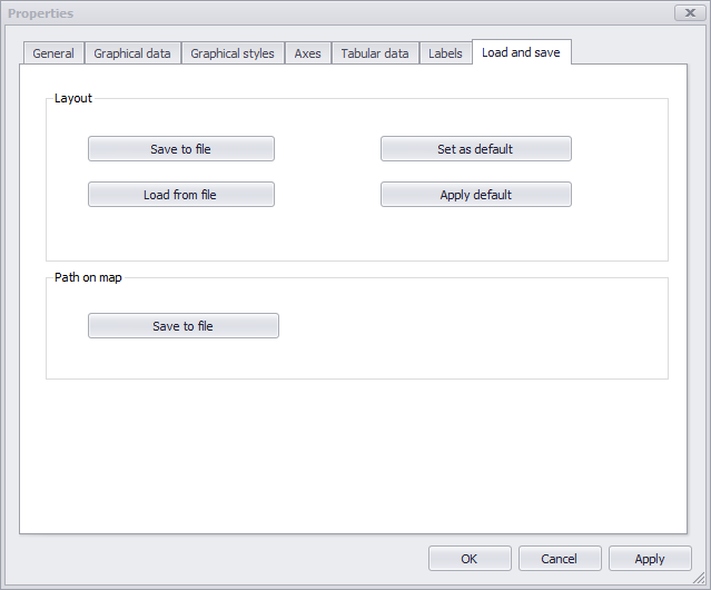
Figure: The Load and Save tab page