Plots and Statistics¶

The 'Plots and Statistics' editor is accessible from the 'Plots and statistics' menu in the 'Setup' tree, or from the 'Calibration plots' button in the 'Results' tab of the ribbon.

This editor allows the user to define relations between externally measured data and simulation results, produce calibration plots, and specify the level of reporting for the calibration.

Identification¶

For each calibration plot, a unique 'ID' must be specified.

The associated measurement station must be specified in the 'Measurement station ID' field. Use the '…' button to pick an ID from a list, or use the arrow button to select the measurement station from the map.

Measured Data¶

The editor contains a Measured Data group where the external time series file (*.DFS0 or *.DAT) and item can be selected.

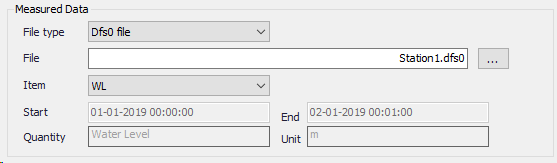
Dfs0 files can be created and edited using the '…' button. They can store multiple measured items in different columns and support various time axis formats. They also contain a definition of quantity type and unit, which is then shown in the editor.

Dat files are text files supporting two different formats.

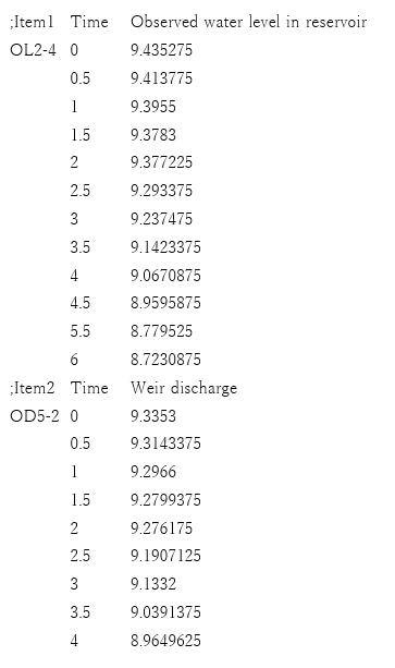
The first format consists in three columns separated by tabs or spaces: Item name, Time and Value. If multiple items are to be stored in the file, they must be provided in the same columns but in consecutive rows. The item name needs to be specified only for its first record and can be left empty for the remaining records. The time should contain a single numerical value with accumulated hours. Comment lines can be inserted and should start with a semicolon. An example is provided below:

The second format for Dat files consists in two columns separated by tabs or spaces: Date-Time and Value. The Date-Time column should be formatted like this: dd/mm/yyy hh:mm.

Result Data¶

The Result Data section is where the result file and item to be compared with the measurement time series is specified.

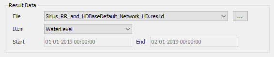
The Result File field takes as default the loaded result file but it is also possible to select the result file manually.

Time series plot¶

In the ‘Time series’ tab in the right panel, the plot shows the superimposed time series of measured and computed data.

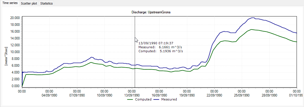
Figure: Comparison of measured and computed time series

The zoom extents can be saved and restored thanks to the use of bookmarks. The bookmarks manager is accessed from a right-click on the time series plot, and contains the following options:

Add: adds a new bookmark, saving the current time extent shown on the plot
Zoom to: zooms to the time period saved for the bookmark selected in the left list
Rename: renames the bookmark selected in the left list
Remove: removes the bookmark selected in the left list
Close: closes the bookmarks manager.

Note

Bookmarks only save the time extent (X axis), but not the extent on the vertical axis, and can therefore be applied to any calibration plots even if they don't all have similar ranges of Y values.

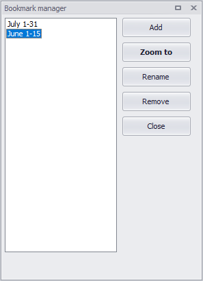
Figure: The bookmark manager from the calibration plots

Scatter plot¶

In the 'Scatter plot' tab in the right panel, the plot shows a scatter plot of the measured and computed values. Each point represents a specific date and time. The computed value of the point is shown on the Y axis, and its measured value on the X axis. The closer the points come to the 45-degree angle line (red line), the closer is the match between measured and computed values.

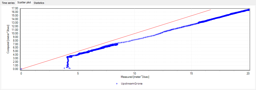
Figure: Scatter plot comparison

Statistics tab¶

In the 'Statistics' tab in the right panel, various statistical values are reported.

In the 'Period' group at the top, it is possible to control the time frame for which the statistics are computed. By default, the statistics are computed for the entire period, but it is possible to change to 'Zoom extent' which computes them for the time span visible in the 'Time series' plot, or to 'Custom period' which computes them for a user-defined period independent from the zoom level in the plot. For the 'Zoom extent' and 'Custom period' options, statistics are computed using values from all time steps within the specified time period. No matter which option is selected, statistics can only be computed for the period where both measured and computed data are available. When computing statistics for the active zoom extent, note that a facility in the Time series plot allows to save and re-use zoom extents (see the 'Bookmarks' option in the context menu of the plot).

In the 'Performance criteria' group, the quantities below are provided to evaluate how well the computed time series fits with the measured time series:

RMSE (Root Mean Square Error): this criterion can be applied as a measure for the magnitude of the deviation between the two time series over the period being investigated.

(25.1)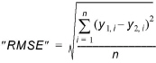

The values for the computed time series are linearly interpolated to get values at the date and times matching the measured data.

Coefficient of determination R2: this is the coefficient of determination, also known as Nash-Sutcliffe efficiency, that measures how well the computed time series matches the measured time series. This criterion is widely used to evaluate model performance in hydrological modelling. It ranges from minus infinity to 1 with larger values indicating a better fit. An important special case is R2 = 0, which can be obtained if the mean measured value equals the mean computed value, indicating that the average of the measured values in this case is as good a predictor as the model. Thus, one would most likely require that R2 > 0 for the model to be fit. The R2 criterion measures the one-to-one relationship between measured and computed values, and hence it is sensitive to bias and proportional effects. It should be emphasized that R2 is based on the sum of squared residuals, and hence provides the same information on goodness-of-fit as the RMSE measure.

(25.2)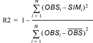

Where OBS is the mean measured value.

The values for the measured time series are linearly interpolated to get values at the same date and times as in the computed data. The calculation of this criterion is valid only when the result file contains a constant time step.

Index of agreement (d): this criterion is not as widely used as E and R2. It ranges from 0 to 1 with large values indicating a better fit. The d measure is also based on the sum of squared residuals, but standardised according to a potential error (the term in the summation in the denominator represents the largest error that each (Computed - Measured)^2 can reach throughout the analysed period). As is the case with E and R2, d is also sensitive to outliers.

(25.3)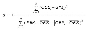

Where OBS is the mean measured value.

The values for the measured time series are linearly interpolated to get values at the date and times matching the computed data. The calculation of this criterion is valid only when the result file contains a constant time step.

Peak time error: this criterion indicates how far in time the two maximum values are located away from each other. This criterion can be used to evaluate if the reported peak values actually compare the same event.
Maximum positive difference: this criterion computes a value indicating how much the computed time series is above the measured time series at the point in time where this difference has its maximum.

(25.4)

The values for the computed time series are linearly interpolated to get values at the date and times matching the measured time series.

Maximum negative difference: this criterion computes a value indicating how much the computed time series is below the measured time series at the point in time where this difference has its maximum.

(25.5)

The values for the computed time series are linearly interpolated to get values at the date and times matching the measured time series.

In the 'General statistics' group, mean values and peak values can also be compared. For each of them, the following values are reported:

Measured: the mean and peak values derived from the measured time series.
Computed: the mean and peak values derived from the computed time series. For the calculation of the mean value, instantaneous values from the computed time series are linearly interpolated beforehand to get values at the date and times matching the measured time series.
Error: the difference of mean and peak values reported for the two time series.
Relative error: the relative difference of mean and peak values, expressed as a percentage of the measured value.

When a time series has a unit which can be accumulated over time (e.g. discharge), the same values are reported for the accumulated values. Typically for a discharge comparison, the table will also report the comparison of accumulated volume.

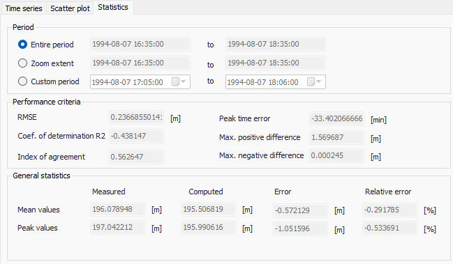
Figure: The calibration statistics results

Statistics button¶

Clicking the ‘Statistics’ button on the Plots and Statistics dialog will open a window providing the overview of results for all the calibration plots, in two different tabs.

The first tab 'Statistics' contains a table with all the statistical values, also provided for the individual plots in their 'Statistics' tab. Note that its columns with "accumulated" values contain data only for the rows associated with a time series with a unit defined "per unit of time" (e.g. discharge).

The second tab 'Global correlation' provides a scatter plot superimposing the sets of points from all calibration plots.

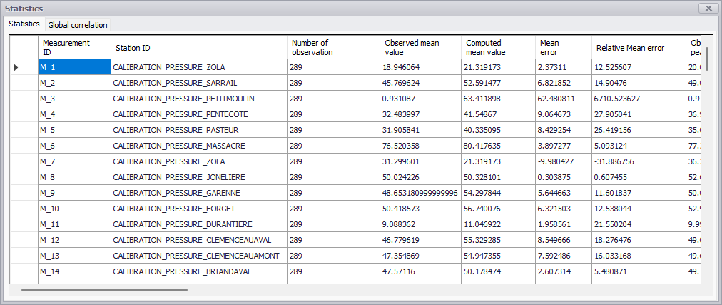
Figure: The global Statistics table

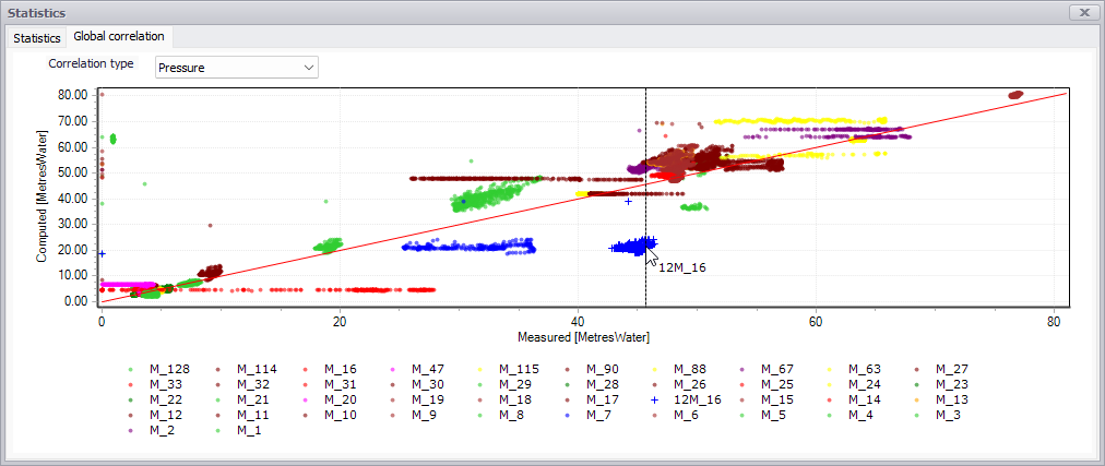
Figure: The global correlation plot

Report¶

The 'Report' button will generate an *.XML report for the currently active calibration plot. It uses a pre-set report template, which includes model description and calibration plots in the report.

The report document can then be exported into various types of document file formats for further use in reports and information dissemination.

Also see the chapter Reports for more details on generating Reports in MIKE+.

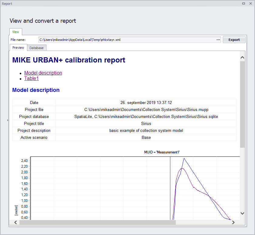
Figure: Example of a calibration report in MIKE+