Result Files¶

The Result Files editor provides a facility for viewing and specifying result file setups in a project. The types or results available depend on the active features and modules for the project (General Settings Model type).

The editor is initially filled with Default result files. These records are distinguished by the “Default_” prefix in their IDs.

The following table shows an overview of the various Default result files that are available in MIKE+.

Default ID	Model Type	Format	Content Type
Default_Surface_runoff	Catchments	.RES1D	Surface runoff
Default_RDII	Catchments	.RES1D	RDII
Default_Storm_water_quality	Catchments	.RES1D	Storm water quality
Default_Storm_water_sediments	Catchments	.RES1D	Storm water sediments
Default_LIDs	Catchments	.DFS0 (currently hard-coded)	LIDs
Default_Catchment_discharge	Catchments	.RES1D	Catchment discharge
Default_Catchment_discharge_quality	Catchments	.RES1D	Catchment discharge quality
Default_Network_HD	Network	.RES1D	Hydrodynamic
Default_Network_RTC	Network	.RES1D	Real time control
Default_Network_AD	Network	.RES1D	Pollution transport
Default_Network_MIKE_ECOLab	Network	.RES1D	MIKE ECO Lab
Default_LTS_extreme_statistics	Network	.RES1D	LTS extreme statistics
Default_LTS_chronological_statistics	Network	.RES1D	LTS chronological statistics
Default_2D_overland	2D Overland	DFSU / DFS2	2D area
Default_2D_overland_AD	2D Overland	DFSU / DFS2	2D area, AD
Default_2D_Flood_statistics	2D Overland	DFSU / DFS2	2D flood statistics
Default_2D_Volume_balance	2D Overland	DFS0	Volume balance

Table: Overview of Default result files

Default result files are initially configured to save results in all model elements, and for the basic result items (calculation parameters).

It is possible to define additional result file setups according to specific modelling needs.

The following properties may be customised for each result file:

File format
Location: Spatial extent or network elements for which results are saved in the file.
Result items: Calculated parameters to be included in the file.

Note

For some content types, only one file format is allowed and cannot be changed.

Info

For 1D networks, multiple result sets comprised of various location-item combinations may be specified for one user-specified result file. See section Defining different locations per result item.

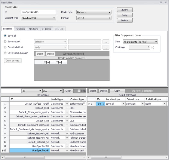
Figure: The Result Files editor

The various tabs and components of the Result Files editor are described in succeeding sections.

Identification¶

The Identification group box on the 'Result files' editor contains general information on a result file item.

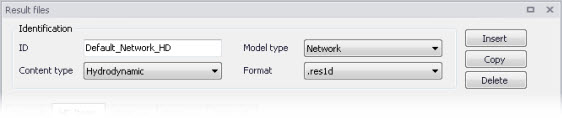
Figure: The Identification group box on the Result Files editor

Model Type¶

Each result file item is categorised based on the type of model from which it is generated. The model may either be a Catchment model, a Network model (comprising CS network and/or River network) or a 2D Overland model.

Content Type¶

This parameter characterises result files according to the calculation modules, and filters the available result items that may be included in the result file setup. The available categories depend on the selected Model Type for a result file setup.

Note

There are also “mixed content” types, which allow flexibility in terms of mixing result items across various active computational modules in one result file setup.

Content Type can be:

For ‘Catchments’ Model Type:
- Mixed catchment contents. Content type for which result items across various active catchment model-related computational modules may be included.
- Surface runoff
- RDII
- Storm water quality
- Storm water sediments
- LIDs
- Catchment discharge
- Catchment discharge quality
- Statistics. For this content type, the result file will save maximum, time of maximum, minimum, time of minimum, and average values for the selected result items. For the relevant result items, it will also save the accumulated values over time (e.g. volume accumulated over time, for a discharge results). This result file contains a single time step.
For ‘Network’ Model Type:
- Mixed content. Content type for which result items across various active network model-related computational modules may be included (e.g. HD, AD, ST, and MIKE ECO Lab).
- Hydrodynamic
- Pollution transport. If the ‘Water Quality (AD)’ module is active.
- MIKE ECO Lab. If the ‘Water Quality (MIKE ECO Lab)’ module is active.
- LTS extreme statistics. If the ‘Long Term Statistics (LTS)’ module is active.
- LTS chronological statistics. If the ‘Long Term Statistics (LTS)’ module is active.
- Statistics. For this content type, the result file will save maximum, time of maximum, minimum, time of minimum, and average values for the selected result items. For the relevant result items, it will also save the accumulated values over time (e.g. volume accumulated over time, for a discharge results). This result file contains a single time step.
- 2D map. This content type provides a 2D result file where results from the 1D simulation are distributed across cross sections and interpolated along the river line. The maps are saved in dfs2 file format (rectangular grids) and constructed through interpolation in space of the 1D grid point results. Thus, the maps constructed in this way should be viewed as a two dimensional interpretation of results from a one-dimensional model.
- State files (initial conditions). State files store results from all active modules in the simulation (Hydrodynamic, Rainfall-runoff, Transport, etc.) and for a given time step. When 'State files' are included in a simulation, there are actually several files saved during the simulation (one per time step, with the saving period selected in the 'Simulation setup' editor). State files are designed to be used as initial condition afterwards, for another simulation. They contain more detailed information than .res1d files and therefore offer more accurate initial condition definitions. Using state files as initial conditions is also activated in the 'Simulation setup' editor, in the 'HD' tab.
- Decoupling. This produces a special hydrodynamic result file, to be used as input for a decoupled Transport (Advection-Dispersion or Water Quality) simulation. The created special hydrodynamic result file stores the simulated water level and the average discharge per saved time step. Decoupling a transport simulation from the hydrodynamic simulation speeds up the simulation by getting the hydrodynamic conditions from the decoupled result file, instead of running the hydrodynamic simulation at the same time. The decoupling of the transport simulation is activated in the 'Simulation setup' editor.
For ‘2D Overland’ Model Type:
- 2D area: a map result file containing instantaneous results at regular time intervals
- 2D flood statistics: a map result file containing a single time step with statistical results (e.g. maximum values over time)
- Time series: time series results from one or more cells from the 2D domain
- Volume balance: a time series providing total volumes over the 2D domain
- Section discharge: a time series providing the total discharge computed through a cross section
- 2D area, AD: a map result file containing instantaneous water quality results at regular time intervals
- Time series, AD: time series of water quality results from one or more cells from the 2D domain
- 2D culverts results: time series of results in selected culverts. The time series will save for each culvert the target discharge (discharge calculated using the empirical formulas), the discharge (effective discharge, which can be less than the target discharge if the upstream water depth is too low), accumulated discharge, and water level on both sides of the culvert (for a short culvert the left and right water level is the mean water level in the real wet elements to the left and right of the section of faces; for a long culvert the start and end water levels are the mean water level in the real wet elements to the right of the two end sections).
- 2D weirs results: time series of results in selected weirs. The time series will save for each weir the target discharge (discharge calculated using the empirical formulas), the discharge (effective discharge, which can be less than the target discharge if the upstream water depth is too low), accumulated discharge, and water level on both sides of the weir (the left and right water levels are the mean water level in the real wet elements to the left and right of the section of faces).
- Section statistics: a *.dfs0 file with a relative item axis, showing the maximum water depth and/or maximum water level in each element face from the mesh, along a defined cross section. The axis of this result file is the index number of the element faces along the cross section.

Format¶

Some result files may be saved in various file formats.

An overview of the Identification group attributes in the Result Files editor is shown in the table below.

Edit field	Description	Used or required by simulations	Field name in datastructure
ID	Unique identifier for the result file setup	Yes	MUID
Model Type	Categorises the model used to generate the result file as either: - Catchment model, or - Network model - 2D overland model	Yes	ModelTypeNo
Content Type	The type of result set under which the result file item falls under.	Yes	ContentTypeNo
Format	The file format for the generated result file is either: - .RES1D -.DFS0 - DFSU - DFS2 - state1d - txt	Yes	FormatNo

Table: Overview of the Identification group box attributes (Table msm_RS)

The buttons to the right of the Identification group box control the data rows in the left overview table in the Result Files editor:

Insert: Adds a new result item in the Result Files table.
Copy: Creates a copy of an active result file item. The ID of the copied item is set the same as the original item’s ID plus the suffix ‘_Copy’.
Delete: Deletes the current selected rows from the left overview table in the editor.

Location¶

The flexibility in results-saving in MIKE+ extends to possibilities for selecting elements or specifying locations for which to save results in the file.

Result locations may be defined for user-specified result files, but not for Default results. Note that Default result files will always save results in all model elements (i.e. ‘Save all’ option).

Result saving locations are specified in the Location tab in the Result Files editor. Available options depend on the type of result file being configured.

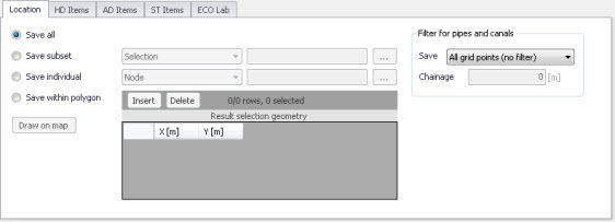
Figure: The Location tab in the Result Files editor

Edit field	Description	Used or required by simulations	Field name in datastructure
[Location radio buttons]	Radio button for selection result saving location: - Save all - Save subset - Save individual - Save within polygon - Save list / all but list	Yes	SelectionNo
[Save Subset dropdown menu]	Dropdown menu for selecting the type of subset	If Location = Save subset	SubsetNo
[Selection list input box]	Input box for a Selection List	If Location = Save subset and Subset = Selection	SelectionListID
[Save Individual dropdown menu]	Dropdown menu for selecting the type of model element for which to save results	If Location = Save individual	IndividualNo
[Element input box]	Input box for an element selection	If Location = Save individual	ElementID
Save [Filter for Pipes and Canals]	Option for selecting the calculation grid point(s) along pipes and canals for which to save results	Yes If Model Type = Network, and results are saved in Pipes and Canals	GridPointNo
Chainage [Filter for Pipes and Canals]	Input box for specifying the chainage (i.e. distance from upstream node) of grid point along the pipe or canal for which to save results	Yes If Model Type = Network, results are saved in Pipes and Canals, and Save = User-specified chainage	Chainage

Table: Overview of the Location tab attributes in the Result Files editor (Table msm_RSS)

Save all¶

This option saves results in all model elements. Note that this option is not available when results are saved in .dfs0 format (see Format section).

Save subset¶

This option offers a dropdown list of possible subset groups for which to save results. The list varies according to Model Type associated with the results. A selection list must be defined (figure below) when the subset is a ‘Selection’.

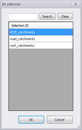
Figure: Selection lists in the ID Selector window

Save individual¶

This option offers a dropdown list of model elements for which to save results. The list varies according to the Model Type associated with the results. An element ID must be defined for the selected model element.

Save within polygon¶

Results from only the network elements or the 2D domain elements within a specified polygon are saved in the file. The polygon is characterised by vertex XY coordinates defined in the secondary grid on the Location tab (figure below).

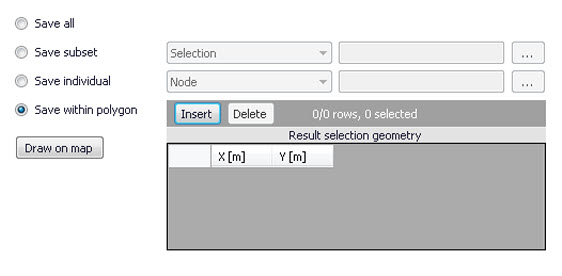
Figure: The Result Selection Geometry secondary grid in the Location tab

The location polygon may be defined by:

Defining values in the secondary table: polygon vertex locations are added and removed from the table using the 'Insert' and 'Delete' buttons at the top of the secondary grid.
Drawing the polygon on the map using the 'Draw on map' button to the left of the table.
- Use the 'Draw on map' button to define a new polygon on the map. The ‘Draw on map’ button activates the Map view (Figure 12.5). Draw a polygon on the map by defining vertex locations. Double-click on the map to finish the polygon editing. The polygon coordinates are then shown in the secondary table in the Location tab of the Result Files editor.
- The 'Draw on map' button is renamed 'Edit on map' as soon as a polygon has been defined and the secondary table is filled.
- Note that the location polygon is shown on the Map only while drawing. The polygon is no longer shown on the map once the polygon has been drawn.
- When the polygon already exists (i.e. when the Location tab secondary table is not empty), the 'Edit on map' button allows for editing the existing polygon. The Map is shown, where polygon vertices may be moved, deleted, or added.

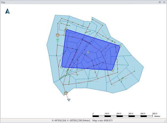
Figure: Defining a result location polygon on the Map

Coordinates¶

For 2D time series data, the X and Y coordinates of the time series must be specified in the table. When multiple coordinates are specified for the same result file, each location will be saved as an individual item in this file. For each time series, the raw results for the 2D domain element in which the coordinates fall will be saved.

For a 2D section discharge result file, coordinates must be specified for the cross section polyline, through which the discharge will be computed.

For a 2D section statistics result file, coordinates must be specified for the cross section polyline, along which the maximum water depths and water levels will be reported.

Defining saving grid points¶

The Filter for Pipes and Canals group box is shown on the right side of the Location tab when the result is from a network model (i.e. Model Type = Network).

This section is used to select grid points along pipes and canals for which results are saved in the result file.

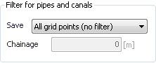
The 'Save' dropdown list offers the following options:

All grid points (no filter)
Upstream grid point
Downstream grid point
Up- and downstream points
Middle grid point
User specified chainage. If ‘User specified chainage’ is selected, specify the grid point location for which results are saved in the 'Chainage' field below. Results are saved for the grid point closest to specified chainage value.

Location of 2D maps¶

For the 2D map content type, the Location tab holds the following information to define the location and the resolution of the rectangular grid on which the 1D results are interpolated.

Cell size: The cell size of the dfs2 result file. The cell size controls the spatial resolution of the map.

Rotation: The rotation of the rectangular grid. The rotation is defined as the angle between true north and the Y-axis of the grid, measured clockwise. When a rotation is applied, the grid is rotated from its lower left corner, i.e. this corner remains at the same coordinates whereas the three other corners are moved.

Extent definition: This controls the way the extent of the map in the two spatial dimensions is defined. Two options are available:

Length: with this option, you specify the width and height of the rectangle to define the dimensions along the two horizontal axes. MIKE+ will derive the extent of the file from the origo and these lengths.
Number of cells: with this option, the user specifies the number of cells of the rectangular grid in the two spatial dimensions.

Lower left corner: The X coordinate (in the first column) and the Y coordinate (in the second column) of the lower left corner of the rectangular grid.

Lengths: The length of the grid along the X coordinate (in the first column) and along the Y coordinate (in the second column). These fields can be edited only when the extent is defined using the option 'Length'. When the extent is defined using the option 'Number of cells', the fields display the lengths which are automatically derived from the number of cells and the cell size.

Number of cells: Number of cells of the grid along the X coordinate (in the first column) and along the Y coordinate (in the second column). These fields can be edited only when the extent is defined using the option 'Number of cells'. When the extent is defined using the option 'Length', the fields display the numbers of cells which are automatically derived from the lengths and the cell size.

The grid may alternatively be defined by drawing the rectangle on the map using the 'Draw on map' button. This button activates the Map view: click and drag on the map to draw the rectangle. Use the icons on the map to move, resize or rotate the rectangle. Right-click on the map to finish editing. The 'Draw on map' button is renamed 'Edit on map' as soon as a grid has been defined.

Note

The grid is shown on the Map only while drawing. The grid is no longer shown on the map once editing is finished.

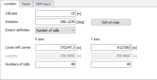
Figure: Defining the rectangular grid for a 2D map result file

Note

The results are mapped only within the extent of cross sections as illustrated in the figure below.

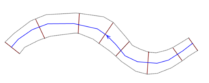
Figure: Illustration of area covered by the 2D map result, based on cross sections extent (red) and river line (blue)

No results will be mapped outside the cross sections extent, and the obtained maps will therefore represent exactly the extent of the flow during the 1D simulation.

An example of a flood map produced through the map-feature is presented in the figure below.

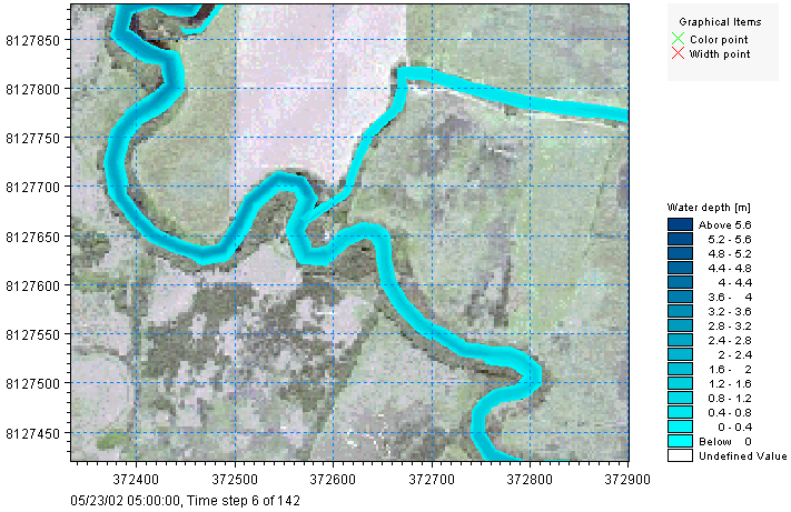
Figure: An example of a 2D water depth map obtained from a 1D river model

Info

2D maps may alternatively be created after the simulation, based on the network result file, and possibly also based on a 2D overland result file, using the Create flood raster tool.

Save list / all but list¶

The 'Save list' and 'Save all but list' options are only available when saving network hydrodynamic results in a .dfs0 or .txt format.

The result file will respectively save all calculation points covered by the table, or all calculation points from the network except those covered by the table. The table is used to define a list of links (pipes or rivers) with upstream and downstream chainages encapsulating all calculation points between these two values.

Note

It is not possible to save these results in .dfs0 or .txt format in nodes or storages.

2D Culverts and 2D Weirs List¶

For '2D culverts results' and '2D weirs results', the location is defined with a list of structures in a table.

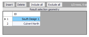
Figure: The list of 2D structures

Use the buttons above the table to add or remove structures from the list:

Insert: Opens the list of valid structures, to select one to add to the table
Delete: Deletes the current selected rows from the list
Include all: Updates the list to save results for all 2D weirs or 2D culverts
Exclude all: Removes all items from the list.

Format¶

When network hydrodynamic results are saved to .txt format, this tab is used to control the format of the created text file.

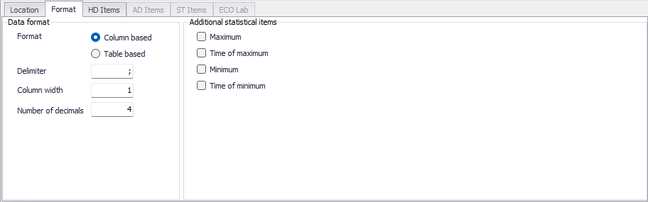
Figure: The Format tab in the Result Files editor

Format¶

Two file formats are available:

Column based: this will generate a text file with a column-based format. There will be one time column and one column for grid point item selected for output. The number of lines will equal the number of saved time steps.
Table based: this will generate a text file with a table-based format. There will be one table for each time step saved. Each table will have rows corresponding to the number of selected grid points, and columns corresponding to the number of selected items.

Delimiter¶

This controls the special character (e.g. semicolon, comma, etc.) to be used between each column.

Colum width¶

This is the desired minimum width of each column. The actual width in the created file will be larger if the content of the column doesn't fit in the minimum width.

Number of decimals¶

The number of decimals written to the file, for result values.

Additional statistical items¶

For each result item saved to the file, it is also possible to save some statistics, including:

Maximum: a separate table at the bottom of the file will show the maximum value of the saved result items.
Time of maximum: a separate table at the bottom of the file will show the time of maximum value of the saved result items.
Minimum: a separate table at the bottom of the file will show the minimum value of the saved result items.
Time of minimum: a separate table at the bottom of the file will show the time of minimum value of the saved result items.

Items¶

Tabs in the 'Result files' editor are used to select items that will be stored in the result file. Different tabs are shown depending on the Model Type and active project Modules.

Note

Customising items related to LIDs is currently not available. Also, modifying items related to MIKE ECO Lab results is done in the MIKE ECO Lab template (.ECOLAB) and not the MIKE+ interface.

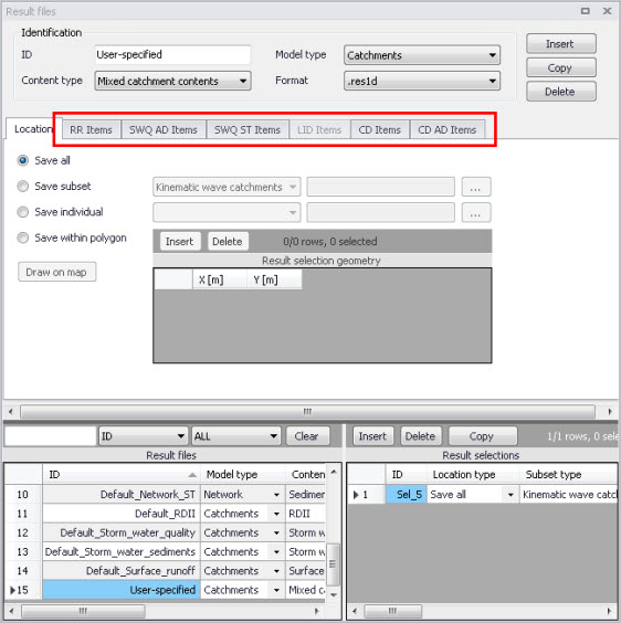
Figure: Item tabs in the Result Files editor. This figure shows available tabs for results from Catchment models.

Each tab shows items related to a computation Module, and the items are categorised as:

Basic items. Primary result parameters for a simulated process.
Additional items. Additional result items that provide greater detail on the simulated processes for the system.

The following sections describe the various result items available in MIKE+.

RR Items (Surface runoff and RDI)¶

These are catchment rainfall-runoff modelling result items.

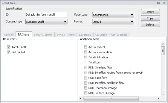
Figure: The RR Items tab in the Result Files editor. The ‘Total runoff’ and ‘Net rainfall’ items are initially included in Default Surface Runoff results.

The table below summarises items that may be saved in surface runoff result files.

Basic Items

Additional Items

Total runoff
Net rainfall

Actual rainfall
Actual evaporation
Total infiltration
RDI: Overland flow
RDI: Interflow routed from second reservoir
RDI: Base flow
RDI: Interflow and base flow
RDI: Rootzone storage
RDI: Surface storage
RDI: Groundwater depth
RDI: Infiltration to groundwater
RDI: Overland first reservoir flow, from first to second reservoir
RDI: Interflow first reservoir flow, from first to second reservoir
RDI: Capillary flux
RDI: Overland first reservoir storage
RDI: Overland second reservoir storage
RDI: Lower base flow
Snow Storage
RDI: Snow ZoneTemperature
RDI: Snow ZoneRainfall
RDI: Snow ZoneWaterRetention
RDI: Snow ZoneMeltingCoefficient
RDI: Snow ZoneAreaCoverage
RDI: Snow ZoneMeltingWater
TimeArea: InitialLossStorage
UHM: Excess Rainfall
KW Runoff [ImperviousSteep, Flat]
KW Runoff [PerviousSmall, Medium, Large]
KW Depth [ImperviousSteep, Flat]
KW Depth [PerviousSmall, Medium, Large]
KW WettingLoss [PerviousSmall, Medium, Large]
KW WettingLoss [ImperviousFlat]
KW StorageLoss [ImperviousFlat]
KW StorageLoss [PerviousSmall, Medium, Large]
KW Infiltration [PerviousSmall, Medium, Large]
KW InfiltrationPotential [PerviousSmall, Medium, Large]
Land use results (see details below)

Table: Overview of Surface Runoff result items in the RR Items tab

Details on Land use results:

Runoff (Kinematic Wave and New UK / Wallingford): this gives the runoff from each land use in the catchment.
Depth on surface (Kinematic Wave): this gives the water depth on each land use in the catchment.
Wetting loss: this gives the wetting loss depth on each land use in the catchment. Not applicable to New UK / Wallingford model type.
Storage loss: this gives the storage loss depth on each land use in the catchment. Not applicable to New UK / Wallingford model type.
Potential infiltration rate: this gives the infiltration rate as computed by the infiltration model (e.g. Horten or Green-Ampt) from each land use in the catchment.
Actual infiltration rate: this gives the actual infiltration rate, which can be smaller than the potential infiltration rate due to insufficient amount of water available on the land use surface.
Potential evaporation rate: this gives the evaporation rate as provided by the input time series or constant value, from each land use in the catchment.
Actual evaporation rate: this gives the actual evaporation rate, which can be smaller than the potential evaporation rate due to insufficient amount of water on the land use surface.
Antecedent Precipitation Index (New UK land use): the API value computed for each land use in a New UK / Wallingford catchment.

SWQ AD Items (Stormwater quality)¶

These are results related to the modelling of water quality of stormwater from catchments.

Figure: The SWQ AD Items tab in the Result Files editor. The ‘Mass transport’ item is initially included in Default Stormwater Quality results.

Basic Items	Additional Items
Mass transport	Mass on catchment surface Accumulated mass transport Concentration

Table: Overview of Stormwater Quality result items in the SWQ AD Items tab

SWQ ST Items (Stormwater sediments)¶

These are results related to the modelling of sediment transport with stormwater over catchments.

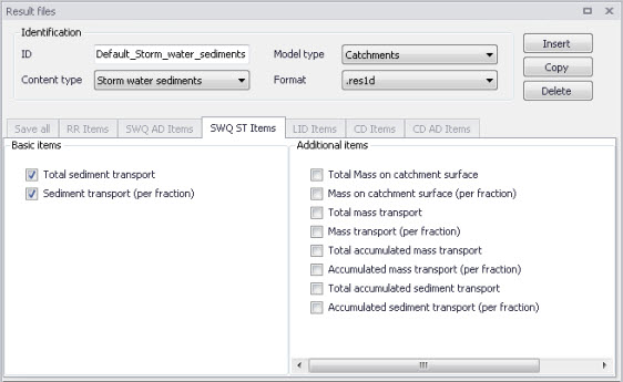
Figure: The SWQ ST Items tab in the Result Files editor. The ‘Total sediment transport’ and ‘Sediment transport (per fraction)’ items are initially included in Default Stormwater Sediments results.

Basic Items	Additional Items
Total sediment transport Sediment transport (per fraction)	Total Mass on catchment surface Mass on catchment surface (per fraction) Total mass transport Mass transport (per fraction) Total accumulated mass transport Accumulated mass transport (per fraction) Total accumulated sediment transport Accumulated sediment transport (per fraction)

Table: Overview of Stormwater Sediments Transport result items in the SWQ ST Items tab

LID Items¶

It is currently not possible to customise result items for LID results in MIKE+. All result items are saved by default. The table below shows the LID result items from a catchment model saved in .DFS0 format.

Basic Items	Additional Items
Rain Inflow Surface Flow Drain Flow Infiltration	Evaporation Surface Depth Soil Moisture Storage Depth Surface to Soil Soil to Storage Drain Storage Depth (Green Roof) Soil to Drain Storage (Green Roof) Pavement Moisture (Porous pavement) Surface to pavement (Porous pavement) Pavement to Storage (Porous pavement) Mass Checksum

Table: Overview of LID result items

Please refer to the ‘LID Deployment Result File’ section under the ‘Rainfall-Runoff Modelling’ chapter for more details on the LID result items listed above.

CD Items (Catchment discharge)¶

Catchment discharge consists of person equivalent (PE)-based or area-based inflows from catchments (e.g. wastewater inflows).

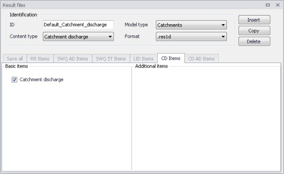
Figure: The CD Items tab in the Result Files editor. The ‘Catchment discharge’ item is initially included in Default Catchment Discharge results.

CD AD Items (Catchment discharge quality)¶

These are computational items related to the modelling of pollutant transport with catchment discharge.

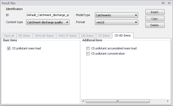
Figure: The CD AD Items tab in the Result Files editor. The ‘CD pollutant mass load’ item is initially included in Default Catchment Discharge Quality results.

Basic Items	Additional Items
CD pollutant mass load	CD pollutant accumulated mass load CD pollutant concentration

Table: Overview of Catchment Discharge Quality result items in the CD AD Items tab

HD Items¶

These are result items related to hydrodynamic calculations in the network, including items related to control rules, which will be saved into the result files during the simulation.

Some additional items related to control rules (setpoint value, pump start level, pump stop level) are always saved even though they are not listed in this tab, because they are essential in case the result file is to be used as hotstart file.

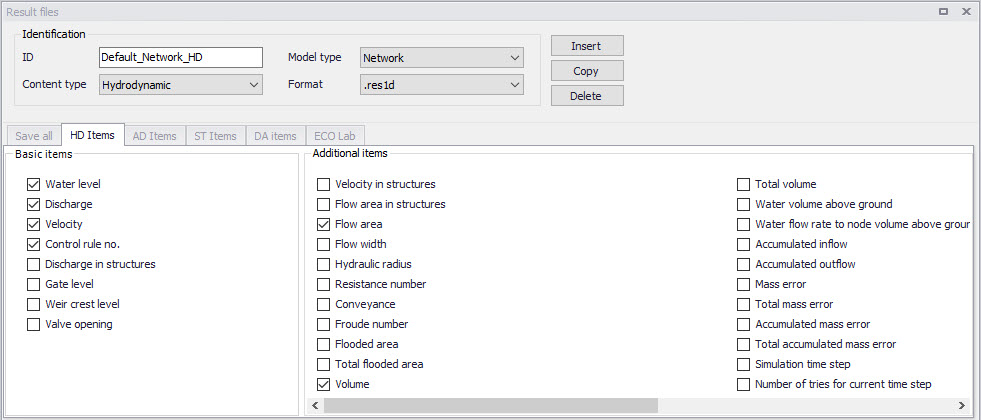
Figure: The HD Items tab in the Result Files editor for network results

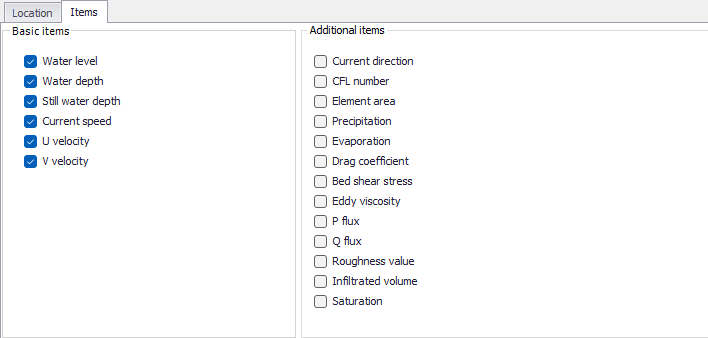
Figure: The Items tab in the Result Files editor for 2D overland results

Note

Some result items are not available when saving to .txt file format, and are therefore disabled.

Details on some of the additional items:

'Weir water level', 'Pump water level', 'Orifice water level' and 'Valve water level' for collection system networks: this gives water level in the two connected nodes on both sides of the weir / pump / orifice / valve.
Mass error: this gives the difference between the calculated and geometric (true) volumes. The calculated volume is evaluated using the inflow/outflow of a grid point at each time step. The geometric volume is evaluated by integrating the width of the cross-section (from its processed data table) from the bottom up to the water level and multiplying by the grid point's length. This result item is called 'Mass error, generated water' in the result file.
Accumulated mass error: this gives the values of 'Mass error' accumulated over time. This result item is called 'Mass error, signed accumulated' in the result file.
Water volume above ground (normal cover nodes): this gives the volume of water stored in the artificial basin, which is introduced above the ground level for nodes with a normal cover, when the water level exceeds the ground level. This result item is therefore only available in nodes with a normal cover. See the Cover description for more information.
Discharge to volume above ground (normal cover nodes): this gives the discharge flowing into the artificial basin, which is introduced above the ground level for nodes with a normal cover. This discharge is positive when the node is surcharging into the basin, and negative when the basin is drained by the network. This result item is therefore only available in nodes with a normal cover. See the Cover description for more information.
Spilling discharge above ground (spilling nodes): this gives the discharge spilling on the surface and irreversibly leaving the model, for nodes with a 'Spilling' cover type, when the water level exceeds the ground level. This result item is therefore only available in nodes with a 'Spilling' cover type. See the Cover description for more information.
Inflow volume stored due to maximum inflow: volume of water stored in the fictive reservoir above nodes defined with a maximum inflow, and temporarily storing the exceeding flows. See Flow Regulation for more information.
Accumulated inflow: this gives the volumes inserted in the model network. It is reported in nodes and links where inflows apply (e.g. from 'Inflow to node' and 'Inflow to link' boundary conditions'), as well as for the entire network. This result item excludes inflows from connected nodes and links, in order to report only inflows from external sources.
Accumulated outflow: this gives the volumes leaving the model network. It is reported in nodes and links where outflows apply (e.g. from spilling nodes, outlets, 'Exfiltration from node' or 'Exfiltration from link' boundary conditions'), as well as for the entire network. This result item excludes outflows towards connected nodes and links, in order to report only flows leaving the modelled network.
Control rule no.: this gives the rule number applied over time for structures regulated using control rules. The reported number represents the rule number shown in the 'Rules' tab from the 'Control rules' editor. Note that this result item is saved for each control rule defined in this 'Control rules' editor, and that multiple control rules can be applied to the same structure (e.g. one control rule controlling a pump's start level and another one controlling its stop level). This result item is primarily designed to be presented in Time Series plots or Results tables. Displaying this result item in a profile plot or a scatter plot does not allow selecting which control rule is plotted, in case multiple control rules exist for the selected structure.
Manhole cover displacement: this gives the cover’s displacement (opening percentage), for nodes with a ‘Displaceable cover’ cover type. The result item is therefore only available in nodes with a ‘Displaceable cover’ cover type. See the Cover description for more information.
Node discharge to surface: for a collection system network coupled to a 2D overland model, this gives the discharge through the coupling at a node, i.e. the discharge from the node to the 2D surface. It is positive when the water flows towards the surface, and negative when the water flows from the surface to the network. This result item is not selectable in the list of items in the 'Result files' editor: it is always saved for coupled simulations.
Node diverted runoff to surface: for a collection system network coupled to a 2D overland model, this gives the part of the catchment runoff which is added as a source inflow in the 2D overland model. This happens when a catchment runoff is inserted in a node, and when this runoff exceeds the maximum discharge specified in the '1D-2D couplings' editor for the node, if any. When this situation occurs, only the maximum flow is added to the node, whereas the exceeding part is assumed to remain on the surface and is added to the 2D overland model, as a source located at the node's place. This result item is not selectable in the list of items in the 'Result files' editor: it is always saved for coupled simulations.
Node water level of coupled model: for a collection system network coupled to a 2D overland model, this gives the water level computed in the 2D overland model at the coupling location, which is used to compute the coupled flow. If the coupling location is defined with a single point (usually corresponding to the node's location), this 2D water level is the water level in the mesh element containing the coupling point. If the coupling location is defined with a polygon shape, this 2D water level is the average water level from all the mesh elements contained in the polygon. This result item is not selectable in the list of items in the 'Result files' editor: it is always saved for coupled simulations.
Link left lateral outfow to surface: for a river network coupled to a 2D overland model, this gives the discharge through the coupling all along the left river bank coupling, i.e. the discharge between the river and the 2D model on the left bank. It is positive when the water flows towards the 2D overland model, and negative when the water flows from the 2D model to the river. This result item is not selectable in the list of items in the 'Result files' editor: it is always saved for coupled simulations.
Link right lateral outflow to surface: for a river network coupled to a 2D overland model, this gives the discharge through the coupling all along the right river bank coupling, i.e. the discharge between the river and the 2D model on the right bank. It is positive when the water flows towards the 2D overland model, and negative when the water flows from the 2D model to the river. This result item is not selectable in the list of items in the 'Result files' editor: it is always saved for coupled simulations.

Besides these selected result items saved to the result files, additional items called "derived items" can be computed in memory while loading the result file for result viewing, for Collection System and River simulations. These derived items therefore do not need to be selected in this editor, although they need their respective source items to be saved. See the Introduction to Results Presentation chapter for more information about how to load derived items from a result file. The following derived items are available:

Node flood: The node flood is calculated as node water level minus node ground level for all nodes except outlets
Node depth: The node depth is calculated as node water level minus node invert/bed level for all nodes
Weir depth, Orifice depth, Pump depth, Valve depth: Water depth in the upstream and downstream nodes of the structure. It therefore provides the same results as the 'Node depth' variable in the connected nodes, but the calculation point location is named according to the structure ID. This is not applicable to structures on a river network.
Node water minus critical level: Calculated for all manholes and basins. For nodes where critical level is specified it is calculated as: Actual node water level - Critical Node level. For nodes where critical level is not specified it is calculated as: Actual node water level - Ground level (i.e. in these places it is equivalent to Node flood)
Link flood: The link flood is calculated as link water level minus link ground level for all links from the collection system network. The link ground level is calculated as: Hground (X) = GroundLevel(upstream node) - ([GroundLevel(upstream node) - GroundLevel(downstream node)]* [Chainage(X) / Length])
Link depth: The link depth is calculated as link water level minus link invert/bed level for each H-point. This invert level is interpolated along pipes, and obtained from the cross section for rivers and natural channels.
Link water minus critical level: Calculated as link water level minus link critical level. The link critical level is calculated as: Hground (X) = GroundLevel(upstream node) - ([CriticalLevel(upstream node) - CriticalLevel(downstream node)]* [Chainage(X) / Length]). For nodes where no critical level is specified, Critical level is replaced by GroundLevel (i.e. it is equivalent to link flood)
Link absolute discharge, Weir absolute discharge, Orifice absolute discharge, Pump absolute discharge, Valve absolute discharge: Absolute value of computed discharge. This is not applicable to structures on a river network.
Link Q/Q of full reach: Ratio between actual (time-varying) discharge and discharge of full reach, where discharge of full reach is the discharge for which the reach gets full, computed using the specified link resistance formulation. The discharge of full reach is constant for each link, and is reported in the summary .html file from the simulation, as well as in result maps when identifying links on the map.
Link filling: Link filling is calculated as the depth divided by the link height, e.g. if the pipe is running under pressure, the ratio will be above 1.0.
Link pressure: Pressure is calculated as water level minus pipe top level (i.e. it is calculated as height of water column above the top of the pipe). It is null when the water level is lower than the top of the pipe. It is not calculated for open cross sections on rivers or natural channels.
Link water minus pipe top level: This is calculated as water level minus pipe top level, no matter if the water level is higher or lower than the top of the pipe. It is identical to the link pressure when the water level is higher than the top of the pipe, but provides negative values when it's lower. It is not calculated for open cross sections on rivers or natural channels.
Link left bank exceedance: this represents the height of water above the left bank of a cross section. It is calculated as water level in the river minus level of marker 1 from the cross section. When the water level is lower than the bank, this result item returns a negative value describing the freeboard. Note that this item is solely computed based on the river water level: in case the river is coupled to a 2D overland model, the actual water depth above the bank may deviate from this result value, typically because the actual bank level may be different than the cross section' marker, or because the water level in the 2D floodplain is higher than in the river bed.
Link right bank exceedance: this represents the height of water above the right bank of a cross section. It is calculated as water level in the river minus level of marker 3 from the cross section. When the water level is lower than the bank, this result item returns a negative value describing the freeboard. Note that this item is solely computed based on the river water level: in case the river is coupled to a 2D overland model, the actual water depth above the bank may deviate from this result value, typically because the actual bank level may be different than the cross section' marker, or because the water level in the 2D floodplain is higher than in the river bed.
Link maximum bank exceedance: this represents the maximum height of water above the left and right banks of a cross section. It is calculated as the maximum between 'Link left bank exceedance' and 'Link right bank exceedance'.

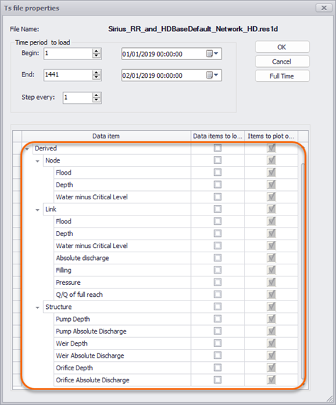
Figure: Example of derived items from MIKE 1D results

AD Items (Pollution transport)¶

These are result items related to the modelling of the transport of pollutants in the sewer network.

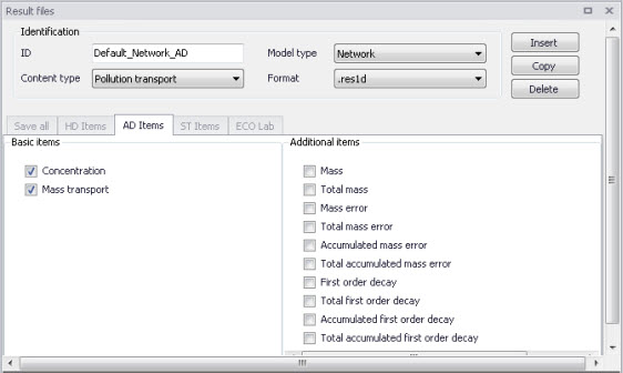
Figure: The AD Items tab in the Result Files editor. The ‘Concentration’ and ‘Mass transport’ items are initially included in Default Pollution Transport results.

Basic Items	Additional Items
Concentration Mass transport	Mass Total mass Mass error Total mass error Accumulated mass error Total accumulated mass error First order decay Total first order decay Accumulated first order decay Total accumulated first order decay

Table: Overview of pollution transport items in the AD Items tab

Note

If the Decay is set to 0 for a component, the decay-related result items which are not relevant for this component are never saved to the result file. That means that decay-related result items are saved only for WQ components with decay different than 0.

MIKE ECO Lab (MIKE ECO Lab water quality)¶

These are the result items from the MIKE ECO Lab simulation. The 'MIKE ECO Lab template' group on the left shows the list of templates included in the project. Select one of the templates to access the selection of result items for this template.

The 'Basic items' group in the center shows the list of state variables and derived outputs from the selected template.

The 'Additional items' group on the right shows the list of auxiliaries and processes from the selected template.

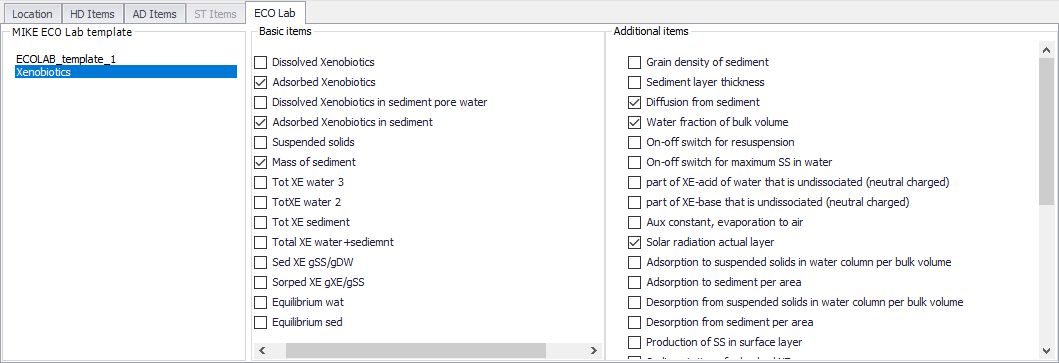
Figure: The MIKE ECO Lab items in the 'Result files' editor

Note

These lists depend on the State Variables, Auxiliary Variables, Processes and Derived Outputs defined in the MIKE ECO Lab template used in the simulation. This template can only be edited in the MIKE ECO Lab editor, in MIKE Zero.

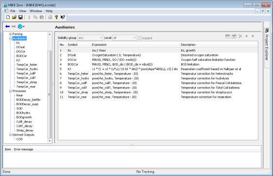
Figure: Example MIKE ECO Lab template (.ecolab) showing the Auxiliaries, Processes, and Derived Outputs sections

LTS HD Items (LTS extreme and chronological statistics)¶

These are LTS statistics results related to LTS hydrodynamic modelling in sewer networks.

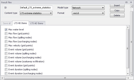
Figure: The LTS HD Items tab in the Result Files editor. The figure shows pre-selected items for Default LTS Extreme Statistics results.

Extreme Statistics

Chronological Statistics

Max water level
Max flow (grid points)
Max flow (spilling nodes)
Max flow (surcharging nodes)
Max velocity (grid points)
Event volume (grid points)
Event volume (spilling nodes)
Event volume (surcharging nodes)
Event volume (soakaway exfiltration)
Event duration (grid points)
Event duration (spilling nodes)
Event duration (surcharging nodes)
Event duration (soakaway exfiltration)

Total accumulated volume (out of the system)
Total accumulated volume (outlet pipes)
Total accumulated volume (pumps out of the system)
Total accumulated volume (weirs out of the system)
Total accumulated volume (orifices out of the system)
Total accumulated volume (valves out of the system)
Total accumulated volume (spilling nodes)
Accumulated spilled volume (spilling nodes)
Accumulated surcharge volume (nodes)
Accumulated exfiltration volume (soakaways)
Accumulated volume (discharge)

Table: Overview of items in the LTS HD Items tab related to LTS Extreme and Chronological Statistics results

LTS AD Items (LTS extreme and chronological statistics)¶

These are LTS statistics results related to LTS modelling of pollution transport in sewer networks.

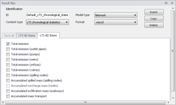
Figure: The LTS AD Items Tab in the Result Files Editor. The figure shows pre-selected items for Default LTS Chronological Statistics results.

Extreme Statistics	Chronological Statistics
Max concentration Event load (grid points) Event load (spilling nodes) Event load (surcharging nodes) Event load (soakaway exfiltration)	Total emission Total emission (outlet pipes) Total emission (pumps) Total emission (weirs) Total emission (orifices) Total emission (valves) Total emission (spilling nodes) Accumulated spilled mass (spilling nodes) Accumulated surcharge mass (nodes) Accumulated exfiltration mass (soakaways) Accumulated mass transport

Table: Overview of items in the LTS AD Items tab related to LTS Extreme and Chronological Statistics results

2D map items¶

This controls the item being mapped in a result file with content type '2D map'. Only one item can be mapped in each file.

Various results items may be mapped:

Water level: this option creates a map of water level. The water level is assumed to be constant along the cross sections, and is then interpolated in the longitudinal direction.
Water depth: this option creates a map of water depth, being the difference between the above water level and the interpolated bed level. This bed level can optionally be defined by a DEM, and is otherwise defined by the cross sections.
Velocity: with this option, the velocity is recomputed based on the water depth in each cell of the grid.
Velocity * depth: this provides a derived result computed as velocity times depth.
DEM: this option generates a digital elevation model (DEM) for the river bed, based on the topography from the cross sections and the river direction.
Depth and fluxes (h, p, q): this option produces a file containing the three items Water depth, P-flux and Q-flux. This map type is primarily used to display flow vectors (using the fluxes information) on top of the water level or depth.
WQ component: this option creates a map of the concentration of the selected component.

Please refer to the MIKE 1D reference manual for details about the mapping procedure.

Besides, three types are available:

Maximum: the overall maximum value throughout the simulation period for each cell included in the map.
Minimum: the overall minimum value throughout the simulation period for each cell included in the map.
Dynamic: time-varying map able to animate the results.

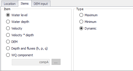
Figure: Selecting the result item for a 2D map result file

Note

For the Velocity item, minimum and maximum results are respectively mapped for the minimum and maximum average velocity in the cross section, and not for the velocity recomputed based on the water depth. As a consequence, the maximum velocity may e.g. occur at low water levels and the map extent may be smaller than for lower velocities.

DEM input¶

An additional option while generating 2D maps of water depth is to include ground level information from external DEM files. In that case, the water levels are mapped to the DEM to compute the water depth, instead of interpolating the ground levels from the cross sections.

To include this option, activate the 'Use input DEM' box.

One or more Digital Elevation Model files must then be supplied in the table. Items are added or removed using the 'Insert' and 'Delete' buttons above the table. The use of multiple DEM files is intended to support multiple DEM tiles to cover the entire area: in that case all the tiles can be supplied in the table, with no need to merge them in a single file. If some files overlap, the topography in the overlapping area will be defined by the first DEM in the list.

Note

The list of DEMs is shared by all 2D map result files i.e., editing the list of DEMs for one 2D map result file will also update any other 2D map result file.

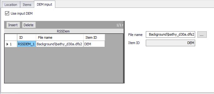
Figure: The optional list of DEMs for 2D map result files

Interpolation¶

For 2D time series results, the spatial interpolation type must be specified.

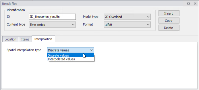
Figure: The Interpolation tab page on the Result Files editor

If ‘Discrete values’ is selected, the values saved to the time series result file are the cell-averaged values.

If ‘Interpolated values’ is selected, the values saved to the result file are determined by second order interpolation. The 2D domain element in which the point is located is determined and the point value is obtained by linear interpolation using the vertex (node) values for the actual element. The vertex values are calculated from the cell-averaged values using the pseudo-Laplacian procedure proposed by Holmes and Connell (1989).

Note

All adjacent elements, including dry elements, are considered in the interpolation calculation.

Defining different locations per result item¶

MIKE+ offers high flexibility in configuring result files obtained from simulations. The secondary table highlighted in the figure below is used to specify different combinations of items and locations for user-specified result setups.

User-specified results (i.e. non-Default) may be configured to contain different result sets with varying combinations of:

Location
Items. Items may be from the same Content Type or from across different (active) Content Types.

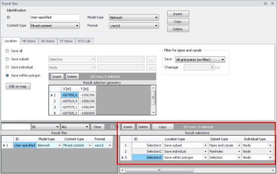
Figure: The secondary table in the Result Files editor

The example shown in this example figure is a ‘Network’ result file setup that has ‘Mixed content’ and includes 3 Location-Items combinations in one .res1d result file. Result items from across content types (i.e. active modules) may also be saved in one file. Use Content Type = ‘Mixed content’ for the result file setup to allow this option.

The Location-Item combinations from this example are summarised in the table below:

Result	Location	Items
Selection1	Save subset = Pipes and canals	HD Items = Water level, Velocity
Selection2	Save individual = Node 7	AD Items = Concentration
Selection3	Save within polygon	HD Items = Discharge

Table: Example Location-Items combinations from across content types that may be combined in one Mixed Content User-Specified result file

The content of the secondary table is controlled with the following buttons:

‘Insert' button¶

Creates a new item in the table, with Default properties.

‘Delete' button¶

Deletes the current selected rows from the secondary table.

‘Copy' button¶

Creates a copy of the active row.