Advection-Dispersion (AD)
Advection-Dispersion (AD) simulates the transport of dissolved substances and suspended fine sediments in the network. Conservative materials as well as those that are subject to a linear decay can be simulated. The computed flow discharges, water levels, and cross-sectional flow areas are used in the AD computation. The solution of the advection-dispersion equation is obtained using an implicit, finite-difference scheme which has negligible numerical dispersion. Concentration profiles with very steep fronts can be accurately modelled. The computed results can be displayed as longitudinal concentration profiles and pollutants graphs, which could be used at the inflow to a sewage treatment plant or an overflow structure. The AD can be linked to Long Term Statistics modelling to provide long-term simulation of pollutant transport.
The option to simulate water age and blend in percentages between two sources can be done with the AD module.
The Advection-Dispersion model can be used to calculate transport of dissolved or suspended substances, age of water, blend in percent between two sources, and for modelling of water temperature variation within the network. The model is based on the one-dimensional transport equations for dissolved materials. The equations reflect two transport mechanisms: the advective transport with the mean flow velocity, and the dispersive transport due to concentration gradients in the water. The transport equations are solved by use of an implicit finite difference scheme, which is fully time and space centred, in order to minimize the numerical dispersion. The main assumptions of the model are:
- The considered substance is completely mixed over the cross-sections. This implies that a source term is considered to mix instantaneously over the cross-section.
- The substance is conservative or subject to a first order reaction (linear decay).
- Fick's diffusion law can be applied, i.e. the dispersive transport is proportional to the concentration gradient.
Special considerations have been given to the transport at manholes and other structures.
The Advection-Dispersion model requires two types of data: time series of concentrations at the model boundaries and data for full definition of the components to be modelled, e.g. initial concentrations, dispersion coefficients and decay rates.
WQ Components
Each of the water quality (WQ) components (substances) to be included in Advection-Dispersion computations must be specified in this section shown in the WQ Components dialog. Naming of component is absolutely flexible, and no ’reserved’ or ’standard’ component names are prescribed.
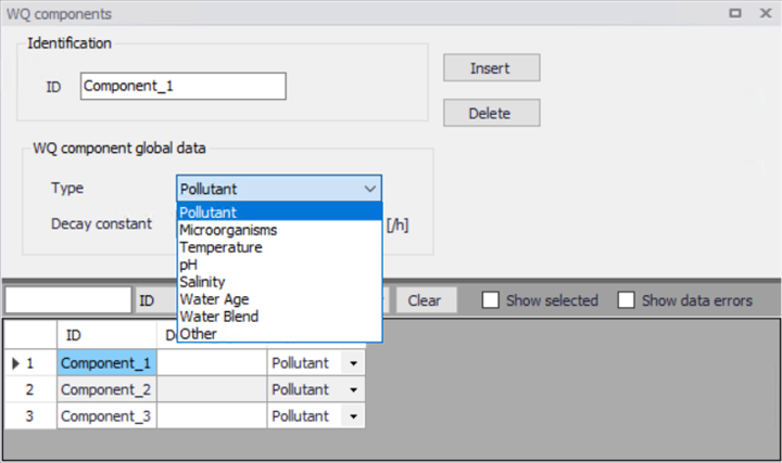
Figure: Define water quality components in the WQ Components editor
The specified WQ components can be declared as 'Pollutant', 'Microorganisms', 'Temperature', 'pH', 'Salinity', ‘Water Age’, ‘Water Blend’, 'Other' or ‘Fixed matter’. This categorization is used for handling of units: each component type has its own list of possible units.
When working with a water quality model using MIKE ECO Lab, each MIKE ECO Lab state variable is associated to a WQ component from this 'WQ component' editor, and the biological processes are controlled by properties defined in the MIKE ECO Lab editors. The 'Fixed matter' type of WQ component is a special type which is relevant for this MIKE ECO Lab models, and is used to describe e.g. components deposited at the bottom and not moving with water.
An optional description of the component can also be specified.
Advection-Dispersion initial conditions for the WQ components can be specified in the AD Initial Conditions editor. Also see chapter AD Initial Conditions. Advection-Dispersion boundary conditions for the WQ components can be specified in the 'WQ boundary properties' editor. Also see Chapter Water Quality Boundary Condition Properties for more description. If not specified otherwise, AD initial conditions and boundary conditions are assumed to be equal to 0.
Info
For coupled 1D-2D models, the defined water quality components are common to both 1D and 2D models. See also WQ components for 2D model.
Decay
For each WQ component a decay coefficient may be specified. The decay coefficient cannot be given for water age and water blend types. A decay set to 0 describes a conservative component, whereas a positive decay describes a non-conservative component. For a non-conservative component, the concentration is assumed to decay according to the first order expression:
(10.1) 
K = the decay coefficient (\(h^{-1}\))
C = the concentration
The decay constant (Decay) is defined as a uniform decay over the entire model for each component.
The decay cannot apply for water age and water blend types. The decay is also not relevant for WQ components associated to a MIKE ECO Lab state variable, for which the decay will be simulated as part of the biological processes modelling.
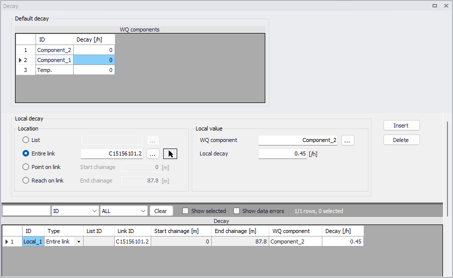
Figure: Define components' decay in the Decay editor
The decay value can be specified either globally using a default value, or locally in parts of the networks (CS and River). The default value will be used at all locations except for locations where local values have been specified. These local values 'overrule' the global specification.
When a local value is located with a list, the specified local decay value applies to all rivers and pipes included in the selected list.
AD Dispersion
The dispersion coefficient is specified as a function of the flow velocity. The function is given as:
(10.2) 
where:
D = the dispersion coefficient (\(\text{m}^{2}/\text{s}\)),
a = the dispersion factor,
u = the flow velocity (m/s),
b = a dimensionless exponent.
If the exponent is set to zero, then the dispersion coefficient is constant and independent of the flow velocity. The unit for the dispersion factor will then be \(\text{m}^{2}/\text{s}\). If the exponent is 1, i.e. the dispersion coefficient is a linear function of the flow velocity, then the unit of the dispersion factor will be meter, and the dispersion factor will in this case be equal to what is generally termed the dispersivity. It is possible to specify values of the minimum and the maximum dispersion coefficients in order to limit the range of the dispersion coefficient calculated during the simulation.
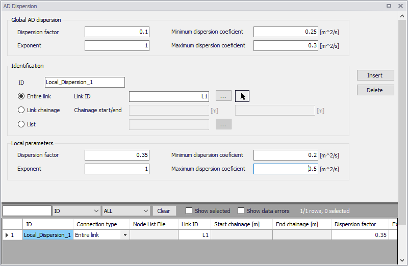
Figure: Define global and local network model dispersion parameters in the AD Dispersion editor.
The dispersion coefficient can be given either globally, or locally in parts of the networks (CS and River).
The global description will be used at all locations except for locations where local conditions have been specified.
The locally specified dispersion coefficients 'overrule' the global specification.